# FAA Vertiport Electrical Infrastructure Study

Federal Aviation Administration Vertiport Electrical Infrastructure Study
Bharatkumar Solanki, Peyton Sanders, Eric Miller,
Priti Paudyal, Bhavesh Rathod, Sherinn Ann Abraham,
Michael Young, Andre Fernandes Tomon Avelino,
Harsha Vardhana Padullaparti, Scott Cary, Chris Hallock,
Kristi Moriarty, Grant Ellwood, Jiyu Wang,
Francisco Flores-Espino, Jayaraj Rane, Tony Markel,
and Anuj Sanghvi
National Renewable Energy Laboratory
NREL is a national laboratory of the U.S. Department of Energy Office of Energy Efficiency & Renewable Energy Operated by the Alliance for Sustainable Energy, LLC
Technical Report NREL/TP-5R00-86245 October 2023
This report is available at no cost from the National Renewable Energy Laboratory (NREL) at www.nrel.gov/publications.
# Federal Aviation Administration Vertiport Electrical Infrastructure Study
Bharatkumar Solanki, Peyton Sanders, Eric Miller,
Priti Paudyal, Bhavesh Rathod, Sherinn Ann Abraham,
Michael Young, Andre Fernandes Tomon Avelino,
Harsha Vardhana Padullaparti, Scott Cary, Chris Hallock,
Kristi Moriarty, Grant Ellwood, Jiyu Wang,
Francisco Flores-Espino, Jayaraj Rane, Tony Markel,
and Anuj Sanghvi
National Renewable Energy Laboratory
## Suggested Citation
Solanki, Bharatkumar, Peyton Sanders, Eric Miller, Priti Paudyal, Bhavesh Rathod, Sherinn Ann Abraham, Michael Young, Andre Fernandes Tomon Avelino, Harsha Vardhana Padullaparti, Scott Cary, Chris Hallock, Kristi Moriarty, Grant Ellwood, Jiyu Wang, Francisco Flores-Espino, Jayaraj Rane, Tony Markel, and Anuj Sanghvi. 2023. Federal Aviation Administration Vertiport Electrical Infrastructure Study. Golden, CO: National Renewable Energy Laboratory. NREL/TP-5R00-86245. https://www.nrel.gov/docs/fy24osti/86245.pdf.
NREL is a national laboratory of the U.S. Department of Energy Office of Energy Efficiency & Renewable Energy Operated by the Alliance for Sustainable Energy, LLC
This report is available at no cost from the National Renewable Energy Laboratory (NREL) at www.nrel.gov/publications.
Technical Report NREL/TP-5R00-86245 October 2023
## NOTICE
This work was authored by the National Renewable Energy Laboratory, operated by Alliance for Sustainable Energy, LLC, for the U.S. Department of Energy (DOE) under Contract No. DE-AC36-08GO28308. Funding provided by Federal Aviation Administration (FAA) Airport Safety R&D Section under IAG-20-17011-0. The views expressed herein do not necessarily represent the views of the DOE or the U.S. Government.
This report is available at no cost from the National Renewable Energy Laboratory (NREL) at www.nrel.gov/publications.
U.S. Department of Energy (DOE) reports produced after 1991 and a growing number of pre-1991 documents are available free via www.OSTI.gov.
Cover Photo from Getty images #1411001016
NREL prints on paper that contains recycled content.
## Acknowledgments
The authors would like to acknowledge the sponsorship of the Federal Aviation Administration (FAA) Airport Safety R&D Section (ANG-E261), which has enabled the collection of content and assessments incorporated within this technical publication. We appreciate the inputs from various aviation industry professionals, including manufacturers, along with the staff and utilities supporting the various sites. We also appreciate the leadership of the FAA’s Wesley Major in providing focus to this work and the review comments from FAA team members including Jonathan Torres, Jeremy Casey, and Darian Byrd were key to providing a quality outcome relevant to the FAA mission.
## List of Acronyms
AC alternating current
ACY Atlantic City International Airport
ANSI American National Standards Institute
BAU business as usual
BESS battery energy storage system(s)
CO2e carbon dioxide equivalent
CRB commercial reference building
DC direct current
DCFC direct-current fast charging
DER distributed energy resource
DISCO Distribution Integration Solution Cost Options DOE U.S. Department of Energy
EPA U.S. Environmental Protection Agency
EVSE electric vehicle support equipment
eVTOL electric vertical takeoff and landing
FAA Federal Aviation Administration
FATO final approach and takeoff area
FBO fixed-base operator
FTE full-time equivalent
GDP gross domestic product
GHG greenhouse gas
GRP gross regional product
HHI Helo Holdings Inc.
HRHC Hard Rock Hotel and Casino
IO input–output
ITC investment tax credit
LPLS Large Power and Lighting – Secondary
LRMER long-run marginal emissions rate
MACRS modified accelerated cost recovery schedule NASA National Aeronautics and Space Administration NPV net present value
NREL National Renewable Energy Laboratory
O&M operations and maintenance
OEM original equipment manufacturer
OLTC on-load tap changer
PSE&G Public Service Electric and Gas Company p.u. per unit
PV photovoltaics
RPC regional purchase coefficient
SRMER short-run marginal emissions rate
TEB Teterboro Airport
UAM urban air mobility
UML UAM maturity level
USEEIO U.S. Environmentally-Extended Input-Output VTOL vertical takeoff and landing
## Executive Summary
Renewed interest in developing and deploying advanced air mobility using vertical takeoff and landing (VTOL) technologies—driven by the electrification of aircraft—has led to the need to define new requirements for planning, designing, and establishing the landing areas and structures intended to service these aircraft (i.e., vertiports and vertistops). One area of interest is the electrical charging needs of VTOL aircraft and the requirements for electrical infrastructure. The Federal Aviation Administration (FAA) has begun to identify the impact of these alternative energy sources on operations and to prepare guidance for communities and city planners to address the unique challenges that novel VTOL aircraft and their supporting infrastructure may bring.
With the introduction of electric VTOL (eVTOL) aircraft, electrical charging loads will be added at the vertiports along with building loads and distributed energy resources (DERs) (Figure ES-1). The key research challenge is the optimization of megawatt-scale building loads, charging loads, energy storage, and renewables production.

Figure ES-1. Airport system optimization showing current challenges.
Source: Illustration by Josh Bauer, NREL (Schwab et al. 2021)
To better understand vertiport infrastructure requirements, FAA identified multiple stakeholders including aircraft manufacturers, electric utilities, potential site property owners, and local communities to evaluate their unique operational needs. Data collection efforts were carried out to attain a holistic understanding of the energy system requirements within and around the vertiport footprint. Six original equipment manufacturers (OEMs) were contacted to obtain key data including aircraft performance, general aircraft information, and cybersecurity.
Several OEMs did not provide any aircraft performance data, and the remaining provided only partial data. In terms of aircraft sizing, all the aircraft fit roughly within a 50 × 50-ft footprint. Direct-current (DC) peak charging power ranges from 300 kW to 1 MW, and surveyed aircraft require 5% or more of onboard energy capacity for takeoffs. These aircraft are considering ground-based liquid cooling during eVTOL charging, and none are considering battery swapping. Considering the received information, vertiports may consider planning for 1-MW (and potentially higher) chargers to align market speed of deployment with utility upgrade timelines. Cybersecurity management was the least complete data source’ it is assumed many details are still proprietary.
The research team at the National Renewable Energy Laboratory (NREL) proposed hypothetical vertiport sites aimed to provide multiple use cases, including locations such as a general aviation terminal (commercial service and reliever), hospital, parking garage, and large heliport. Accounting for these use cases, the research team reached out to the potential sites to request data on utility usage, electrical drawings, historical energy loads, greenhouse gas (GHG) emissions, resilience, cybersecurity, and known environmental, technological, or human hazards. All the potential sites provided annual utility bills, and some provided information about their existing electrical systems and on-site generators. Other key details such as feeder models were not provided.
Determining the electric load demands associated with introducing these aircraft is the first step in finding a cohesive solution for all parties. Potential flight routes were derived, taking into account potential vertiport sites, and drawn in Google Maps as airspace route planning continues to evolve. Aircraft energy consumption was calculated using a physics-based model and considering aircraft parameters, routes, and range of passengers as inputs. Total vertiport operation—including flight schedule and charging demand—was determined using an agentbased model and considering calculated aircraft and vertiport energy consumption, passenger demand schedule, estimated fleet of aircraft, and identified charging infrastructure. Charging demand was determined for two scenarios: (1) constrained, with three chargers at each site (maximum charging rate of 900 kW per site), and (2) unconstrained, with an unlimited number of chargers per site (maximum charging rate of 13.3 MW per site). This highlights the importance of identifying the necessary number of chargers and charging strategy for potential vertiport sites.
Based on charging demand determined for each site, the research team at NREL performed three key analyses: grid impact, on-site generation techno-economic analysis, and GHG emissions impact analysis due to eVTOL charging load. Each analysis considered three scenarios: business as usual (BAU) (without eVTOL charging), BAU including charging demand, and BAU including charging demand and on-site renewable generation. Jobs and economic development, as well as a hazards analysis, were also examined.
Grid impact analysis provided insights into the feeder operating conditions under given scenarios of electric vehicle support equipment (EVSE) infrastructure and DER adoption and evaluated upgrade costs. In the absence of actual utility feeder models, realistic test feeders were selected. Synthetic Models for Advanced, Realistic Testing: Distribution Systems and Scenarios (SMART-DS) data sets provided realistic, large-scale U.S. electrical distribution models for testing advanced grid algorithms and technology analysis. Grid impact analysis found that for all sites, increased demand due to the addition of charging can cause undervoltage situations,
overloading the distribution line(s) and transformers. Thus, to accommodate the addition of such charging demand, grid infrastructure needs to be upgraded or an energy storage system needs to be installed. This highlights the importance of performing grid impact analysis for potential vertiport sites to ensure charging demand can be accommodated without affecting grid infrastructure and power supply.
On-site generation potential was identified via a techno-economic analysis of opportunities for on-site solar photovoltaics (PV) and/or battery storage to support energy goals (e.g., energy cost savings, resilience, clean energy targets), focusing on possible future electrified aircraft scenarios. Charging demand significantly affects utility costs due to demand charges, which are based on peak demand consumption. However, this creates an opportunity for on-site generation with microgrid systems. Techno-economic analysis found potential economic savings by adding PV and battery energy storage systems (BESS).
GHG emissions were calculated based on total energy consumption attributable to each site with and without eVTOL charging demand. Calculations utilized each site’s current energy generation mix and an alternate calculation assuming renewable energy. Avoiding grid-sourced electricity (by offsetting additional eVTOL charging loads with solar PV) results in avoided GHG emissions. Given these constraints, these FAA sites could further reduce or avoid GHG emissions with strategic timing of eVTOL charging paired with PV+BESS dispatch optimized for GHG emissions reductions.
Job and economic development analysis was also performed to estimate the economic impact of urban air mobility electrification projects in New Jersey, New York, and throughout the United States. Input–output analysis is one of the most commonly used and straightforward frameworks to estimate economic impacts from a change in demand in a region, and this study relied on the 2019 U.S. Environmentally-Extended Input-Output state models. The analysis found that grid expansion, charging infrastructure, and microgrid investments can add up to millions of dollars to local gross domestic product (GDP), as well as significant jobs during construction and operations and maintenance for New Jersey and other part of the United States.
Finally, hazard analysis was carried out considering the EVSE infrastructure and associated hazards due to environmental, human, and technological factors. This can help operators identify the correct mitigation practices and appropriate site selection, which will differ depending on the location of the site and various other factors including severity of the hazard. Note that a separate report will focus specifically on these hazards, listing specific applicable standards and codes concerning EVSE infrastructure. There will also be separate reports highlighting cybersecurity concerns and approaches to mitigate such concerns.
This report presents a first-of-a-kind study analyzing the potential impacts of eVTOL charging infrastructure, considering data collected from key OEMs and potential vertiport locations. The study is limited by data received and assumptions made for conducting various analyses but establishes a foundation for carrying out remaining significant future work. The NREL team plans to work closely with FAA and other prospective key stakeholders to further refine the data and provide key analysis accounting for various charging strategies, charging scenarios, and use cases.
## Table of Contents
Executive Summary ... .... v
1 Introduction...... ........ ... 1
1.1 The Vertiport System ...... ............................................................ ...... 3
1.1.1 Vertiport Infrastructure and Operations .................................................................... ....... 3
1.1.2 Current State of Vertiport Design ........................................................................... ......... 6
1.2 eVTOL Aircraft......... ........................................................ ..... 12
1.3 Vertiport Electrification ........................................................................................................1.3.1 Electric Charging Infrastructure and Operations...................................................... ..... 13..... 13
2 Methodology .................... ........... ....................................................................................................... 14
2.1 Site Classification and Assessment ... ....................................................................... ..... 14
2.1.1 Vertiport Site Selection ..... ...................................................................... ..... 14
2.1.2 EVSE Site Selection... .... 19
2.1.3 2.1.4 Generating Site Electricity Demand........Generating Grid Modeling Scenarios...... ................................. ..... 20..... 20
2.2 2.1.5 Estimating Distribution Grid Infrastructure Investments ........................................Summarizing eVTOL Aircraft Operational Criteria and Route Planning Assumptions ...... .... 21.... 22
2.2.1 Operating Criteria...... ... 22
2.2.2 Route Generation...... ................. .. 24
2.2.3 Flight Demand and Scheduling........... ............................ ..... 25
2.3 Estimating On-Site Generation and Storage Opportunities (REopt).................................... ...... 26
2.3.1 Introduction to REopt......... .................................. ..... 26
2.3.2 Resilience Assessment Considerations . ... 27
2.3.3 Economic Considerations.. ..................................................... ... 27
2.3.4 2.3.5 Technology Considerations........................REopt Analysis Process and Scenarios ...... ........................................................... ...... 29...... 31
2.3.6 Site Electric Load and Electric Tariff Summary ...................................................... ..... 33
2.4 Estimating Greenhouse Gas Emissions....... ............................................ .... 37
2.4.1 Defining the Boundary of the GHG Assessment ................................................... .... 37
2.4.2 Analysis Scenarios ............. ........... ........................................................... ...... 37
2.4.3 GHG Emissions Accounting Methods ...................................................................... ..... 38
2.5 Hazards and Risk Analysis... ........................................................ ..... 40
2.5.1 Electric Vehicle Supply Equipment Hazards . .............................................. .... 40
2.5.2 Cybersecurity Evaluation . ........................................... .... 41
2.6 Estimating Economic and Job Impacts ...... ............................................................ ..... 41
2.6.1 Approach and Data..... ........ ................................................................................. ..... 42
3 Results ....... .................................................................... 47
3.1 Vertiport Electrical Infrastructure Upgrade Needs...................................................................... 47
3.2 eVTOL Aircraft Charging Demand ........ .............................................. .... 52
3.3 Electrical Grid Impacts........... ........................................... .... 58
3.3.1 Analysis of the Feeders with ACY and HRHC ........................................................ ..... 59
3.3.2 Analysis of the Feeder With TEB ..... ......................................................... ..... 69
3.3.3 Analysis of the Feeder With HHI. ....................................................................... 75
3.4 Generation and Storage Opportunities (REopt) ...... ........................................................... ...... 79
3.5 Greenhouse Gas Emissions Impacts... ........................................................ .... 90
3.5.1 Summary of Results ........ ...................................................................... ..... 90
3.6 Hazard and Cybersecurity Analysis ............................................................................................ 963.7 Job and Economic Development Impacts ................................................................................... 96
4 Discussion and Conclusion ............................................................................................................ 108
References ............................................................................................................................................... 113
Bibliography .......Further Reading . .................................................................................................................................................................... ..... 119..... 120
## List of Figures
Figure ES-1. Airport system optimization showing current challenges. ..... .. v
Figure 1. Overall analysis methodology. ............. . 2
Figure 2. Isometric operation view of a representative urban air mobility operations environment. . . 3
Figure 3. UAM maturity scale. ..... . 4
Figure 4. Vertidrome airspace boundary............. ........ ............ ........ . 5
Figure 5. Vehicle states within the terminal airspace. .................................................................... .... 6
Figure 6. FAA vertiport dimensions. .... ............................................................. .. 8
Figure 7. Vertiport perimeter lighting.. .................... . 9
Figure 8. FAA vertiport rooftop example. .......... ........ . 10
Figure 9. Lilium’s urban vertiport layout with (a) takeoff area, (b) parking stands, and (c) terminal. .. 11
Figure 10. Example of an on-airport vertiport. ....... ... .. 12
Figure 11. ACY transformer and potential vertiport locations. .... ................................................ . 15
Figure 12. TEB general vertiport proposed site...... .......................................................................... . 16
Figure 14. HHI public helipad. .......... ......... .................................... . 17
Figure 16. AtlantiCare facility and helipad.. ......... ................................... .. 18
Figure 17. Hard Rock Hotel and Casino....... . 18
Figure 18. DISCO tool: automated distribution grid upgrades. ..... ................................. . 22
Figure 19. Methodology applied to determine charging demand. ................................ . 23
Figure 20. Altitude vs. distance traveled on the route between ACY and HRHC. .................... . 25
Figure 21. Route between ACY and HRHC. . ......... .......... . 25
Figure 22. Third-party ownership model as implemented in REopt... . 29
Figure 23. Steps taken as part of the REopt analysis for sites. ....... .................................... ..... 31
Figure 24. Average energy prices used for TEB modeling.. ........................................ . 34
Figure 25. Average monthly energy prices for ACY per electric bills. . ........................................... . 35
Figure 26. Plot of hourly energy charges used as HHI’s energy rate. .... ............................... .. 36
Figure 27. Economic impact analysis overview. ..... .............................................. . 42
Figure 28. Total investment by site and category. ............. ............................................................ .. 44
Figure 29. Annual O&M costs by site and category.. .. . 46
Figure 30. Ownership models for different infrastructure. ..... . 50
Figure 31. Average energy consumed by aircrafts for different routes with different numbers of
passengers. .... . 52
Figure 32. Example eVTOL parking and takeoff and landing area at ACY.... .... 53
Figure 33. Example eVTOL parking and takeoff and landing area at HRHC. . . 54
Figure 34. Likelihood/weight assigned for (a) origin/destination, (b) party size at different origins, and (c)
time of request at different origins. ...... . 55
Figure 35. Wait times for passenger demand for both constrained and unconstrainted charging stations. 56
Figure 36. Vehicle airborne time achieved for passenger demand for both constrained and unconstrainted
charging stations. ..... ........ 57
Figure 37. Charging demand profile for ACY with constrained and unconstrained charging station
scenarios.. . 57
Figure 38. Energy dispensed for charging at different sites for unconstrained charging stations. . .. 58
Figure 39. Energy dispensed for charging at different sites for constrained charging stations. ...... ........ 58
Figure 40. Two test feeder networks with ACY and HRHC sites (blue network referred to as Feeder A
and pink network as Feeder B)...... .. 59
Figure 41. (a) Feeder total active and reactive power and (b) overall voltage with and without eVTOL
charging loads considering all nodes in the feeder (Feeder A includes parts of ACY). ........ 60
Figure 42. Peak time voltage heat map on the Feeder A network for (a) BAU and (b) BAU+CH. ........... 61
Figure 43. (a) Feeder total active and reactive power and (b) overall voltage with and without eVTOL
charging loads considering all nodes in the feeder (Feeder B includes HRHC and part of
ACY). .... ...... 62
Figure 44. Transformer loading on the peak day at (a) the HRHC site and (b) the ACY site on Feeder B... 62
Figure 45. Thermal and voltage violations for Feeder A with eVTOL charging load and part of ACY. ... 64
Figure 46. Thermal and voltage violations for Feeder B with eVTOL charging load, HRHC, and part
of ACY. .......... .................. 65
Figure 47. Feeder A with ACY (a) total active and reactive power; (b) overall feeder minimum,
maximum, and average voltage per unit; and (c) site transformer loading percentage
with the deployment of energy storage. ............ ......... 67
Figure 48. Feeder B with ACY and HRHC (a) total active and reactive power and (b) overall feeder
minimum, maximum, and average voltage per unit....... ........ 68
Figure 49. ACY site with energy storage in Feeder B (a) voltage per unit and (b) transformer loading.... 69
Figure 50. Feeder total power (includes TEB) in the BAU scenario for the (a) yearly profile and
(b) peak day profile. .................. ..... 69
Figure 51. Feeder total power with and without eVTOL charging loads (includes TEB). ................ ......... 70
Figure 52. Feeder overall voltage with and without eVTOL charging loads considering all the nodes
in the feeder (includes TEB). ....... ........... 70
Figure 53. Feeder network heat map showing the peak time per unit voltage with the eVTOL charging
scenario. . ... 70
Figure 54. Existing TEB site transformer loading with and without eVTOL charging loads. ... 71
Figure 55. Thermal and voltage violations in feeder due to eVTOL charging loads (including TEB)
that require infrastructure upgrades. ........ ................ 72
Figure 56. With eVTOL charging loads and energy storage deployed: (a) feeder total active and
reactive power; (b) overall minimum, maximum, and average voltage; and (c) TEB site
transformer loading. ............. ................. 74
Figure 57. Feeder with HHI (a) total active and reactive power and (b) overall minimum, maximum,
and average voltage per unit considering all the nodes in the feeder..... ... 75
Figure 58. HHI site (a) node voltages and (b) transformer loading on the peak day. . 76
Figure 59. Thermal and voltage violations for the HHI feeder........................... ...... 77
Figure 60. Time-series profile with energy storage addition: (a) feeder total power and (b) overall
minimum, maximum, and average voltage considering all the nodes in the feeder. ...... . 78
Figure 61. HHI site existing transformer loading with energy storage integration.. . 79
Figure 62. Example of solar PV and BESS dispatch to meet site loads at ACY under the restricted
rooftop area scenario. ..... .. 84
Figure 63. Monthly peak demand values at TEB for various scenarios. . 84
Figure 64. Monthly peak demand values at ACY for various scenarios.. .. 85
Figure 65. Monthly peak demand values at HHI for various scenarios.... . 85
Figure 66. Visualizing the probability of survival for all optimal scenarios for all three sites........ .. 90
Figure 67. Grid electricity emissions rates for New Jersey, 2024–2050........... . 91
Figure 68. Attributional accounting of GHG emissions from electricity consumption at ACY.. . 93
Figure 69. Attributional accounting of GHG emissions from electricity consumption at TEB. . 95
Figure 70. Attributional accounting of GHG emissions from electricity consumption at HHI. . .. 96
Figure 71. Total construction impacts by category, ACY. .... .. 98
Figure 72. Total construction impacts by category, TEB. ............... . 99
Figure 73. Total construction impacts by category, HHI heliport. .......................... .. 99
Figure 74. Total construction impacts by category, HRHC. .......................... 100
Figure 75. Total earnings by category, sector, and region. ..................................................................... 101
Figure 76. Total O&M impacts per year by category, ACY.............................................................. 102
Figure 77. Total O&M impacts per year by category, TEB........ . 102
Figure 78. Total O&M impacts per year by category, HHI heliport... . 103
Figure 79. Total O&M impacts per year by category, HRHC. . . 104
Figure 80. Total annual earnings by category, sector, and region. . 105
Figure 81. Total construction impacts by category, average. ...... . 106
Figure 82. Total O&M impacts per year by category, average............ . 107
## List of Tables
Table 1. Vertiports and Vertistops Considered. . 24
Table 2. REopt Economic Assumptions . . 28
Table 3. Solar PV Assumptions in REopt. . 30
Table 4. BESS Assumptions in REopt........ . 31
Table 5. Summary of Scenarios Evaluated in REopt for Each Site . . 32
Table 6. PSE&G LPLS Rate Schedule Breakdown.. . 33
Table 7. Breakdown of Atlantic City Electric’s Annual General Service – Secondary (AGS) Rate
Schedule..... . 34
Table 8. Breakdown of Energy Charges Used for ACY.. . 34
Table 9. Breakdown of General Light and Power Rate Schedule and BGS Energy (Utility Company)
Charges Used for HHI.. . 36
Table 10. Expense Allocation Assumptions ... .. 44
Table 11. O&M Yearly Cost Assumptions.. . 45
Table 12. Vertiports Considered in the Simulation. . 54
Table 13. Example Passenger Demand Schedule . . 56
Table 14. Grid Performance Metrics Comparison for the Peak Day (Feeder A).. . 61
Table 15. Grid Performance Metrics Comparison for the Peak Day (Feeder B). . 63
Table 16. Grid Parameters BAU+CH, After Infrastructure Upgrades and With Energy Storage for Feeder
A. The values in red show the violations observed in the feeder.. . .... 64
Table 17. Grid Parameters BAU+CH, After Infrastructure Upgrades, and With Energy Storage for Feeder
B. The values in red show the violations observed in the feeder. .. 66
Table 18. Grid Performance Metrics Comparison for the Peak Day . . 71
Table 19. Grid Parameters BAU+CH, After Infrastructure Upgrades, and With Energy Storage for TEB
Feeder. The values in red show the violations observed in the feeder.. .. 72
Table 20. Grid Performance Metrics Comparison for the Peak Day (Feeder With HHI). Red values
represent unacceptable results.... .. 76
Table 21. Grid Parameters BAU+CH, After Infrastructure Upgrades, and With Energy Storage for HHI
Feeder. The values in red show the violations observed in the feeder.. ..... 77
Table 22. Site Information and Key Electricity Cost and Consumption Data Extracted From Provided
Utility Bills........ 80
Table 23. A Comparison of BAU and BAU+CH Scenario Shows the Impact of EVSE and Charging
Loads on Each Site’s Electric Utility Charges and Electricity Consumption Trends ...... .... 81
Table 24. Changes in Peak Demand Determination Time Frames with EVSE Loads ..... . 82
Table 25. Optimal System Sizes for Optimal and optimal\_restricted Scenarios Run for Each Site.. .. 83
Table 26. Comparison of Financial Results for ACY’s BAU+CH and Optimal Scenarios..... . 86
Table 27. Comparison of Financial Results for ACY’s BAU+CH and Restricted Optimal Scenarios ...... 86
Table 28. Comparison of Financial Results for TEB’s BAU+CH and Optimal Scenarios . . 87
Table 29. Comparison of Financial Results for TEB’s BAU+CH and Restricted Optimal Scenarios ....... 88
Table 30. Comparison of Financial Results for HHI's BAU+CH and Optimal Scenarios..... . 89
Table 31. Optimal Systems With High-Power, Short-Duration Batteries Do Not Provide Very High
Probability of Surviving 4-Hour Outages . .. 90
Table 32. Materials and Services Sourcing Scenarios ... . 97
## 1 Introduction
The development of civil heliports (places where helicopters takeoff and land) began primarily in response to the needs of businesses in rural and urban areas. Recently, there has been increasing attention focused on the development and deployment of advanced air mobility involving vertical takeoff and landing (VTOL) technologies, driven by the electrification of aircraft at these heliports. This renewed interest has led the Federal Aviation Administration (FAA) to begin studying ways in which new rotor configurations, along with alternative energy sources, will impact operations. Thus, in order to better prepare communities and city planners for the unique challenges that VTOL aircraft and the supporting infrastructure may bring, FAA is beginning to develop guidance around what are now being defined as vertiports and vertistops.
A “vertiport” is defined by FAA as “an area of land, or a structure, used or intended to be used, for electric, hydrogen, and hybrid VTOL aircraft landings and takeoffs and includes associated buildings and facilities” (FAA 2022). Vertiports may operate similar to heliports. However, vertiports may have the capability to serve a wider variety of aircraft configurations and propulsion systems. Vertiport locations will depend on VTOL use cases and could be sited at existing airports or heliports, on rooftops, or at other locations as needed. The vertiport will serve not only as a takeoff and landing location, but also as a location for charging VTOL aircraft with electric propulsion systems.
Alternatively, vertistops are minimally developed vertiports with touch-and-go designs. Boarding and deboarding of passengers and/or cargo is the primary and “minimal necessary operation” that occurs at a vertistop, and with quicker turnaround times, the opportunity to charge aircraft at vertistops is unlikely to be justified (Schweiger and Preis 2022). When comparing the services and capacities at each location, it is helpful to think of the vertiport– vertistop relationship similar to that between a bus terminal and bus stop (Vascik 2020).
The introduction of electric or hybrid electric VTOL aircraft at vertiports will necessitate increasing electric power services and fundamentally changing the approach toward infrastructure sizing. In many situations it has been common practice to size electrical infrastructure for peak demand. This ultimately leads to underutilized infrastructure and higherthan-necessary capital costs when most often vertiport operations do not exceed average energy consumption. To be more cost- and resource-efficient, alternative system designs that include battery energy storage systems (BESS), on-site generation, or a microgrid have become increasingly popular design considerations. Moving away from traditional design practices and incorporating new technologies has been vital for increased resilience on-site and in neighboring communities. Some of these practices and technologies, like net metering services, can also help to generate profit by feeding electricity back to the local electrical grid (Frithiof, Jonat, and Le Bris 2022).
Overall, constructing the necessary vertiport infrastructure requires the collaboration and cooperation of multiple stakeholders including aircraft manufacturers, electric utilities, potential site property owners, and local communities. Each of these entities has their own unique operations and needs to be evaluated, which is why understanding the electric load demands associated with introducing these aircraft is the first step in finding a cohesive solution for all involved parties. Therefore, the National Renewable Energy Laboratory (NREL) has begun data collection efforts to attain a holistic understanding of the energy system requirements that exist within and around the vertiport footprint. Figure 1 presents the overall analysis methodology considering data collection and respective key inputs and outputs from different studies and analysis.

Figure 1. Overall analysis methodology.
Based upon the use cases and data collected, NREL has completed analysis that anticipates challenges and identifies potential solutions for electrified vertiport infrastructure with a focus on the following areas:
Identifying charging infrastructure requirements based on estimated electric vertical takeoff and landing (eVTOL) aircraft fleet sizes, potential use cases, charging strategies, and existing facility infrastructure and constraints.
Recommending electric vehicle support equipment (EVSE) locations based on load profiles and any identified physical and electric infrastructure constraints for eVTOL aircraft charging.
Identifying opportunities for on-site power generation, primarily considering solar photovoltaics (PV) and BESS.
Evaluating hazards and risk characterization involving power systems, battery storage, cybersecurity, and EVSE infrastructure.
Determining greenhouse gas (GHG) emissions based on total energy consumption using (1) current generation and (2) renewable energy at each site.
The act of identifying and overcoming the unique challenges associated with the supporting infrastructure of electrified aviation is a common pursuit occurring among other aeronautical and aviation partners. In one current example, NREL and researchers from the National Aeronautics and Space Administration (NASA) and Georgia Institute of Technology are considering electricity costs and flight demand to study the impacts of regional air mobility and a broader
range of electrified aircraft on electric infrastructure at airports. Yet before electric aircraft can be integrated into the U.S. aviation system, more research is needed. Ongoing and future research with FAA and NASA will ultimately allow for communities and regional transportation systems to potentially reap the benefits of increased mobility, decreased regional travel costs, reduced ground operational emissions, and the decentralization of renewable energy hubs among airports and vertiports.
Through this study, market barriers (such as regulatory hurdles) involving uncertainty in standards and operational requirements of eVTOL aircraft or vertiport infrastructure will be potentially reduced. Defining systemwide best practices in charging systems and facility layouts will allow manufacturers, airports, and communities to be better prepared to participate in this emerging industry.
## 1.1 The Vertiport System
## 1.1.1 Vertiport Infrastructure and Operations
As part of advanced air mobility, specifically an urban air mobility (UAM) vision shared by several public agencies and private industry partners, the vertiport is a critical terminus for sequencing and spacing of aircraft throughput in various airport and metropolitan ecosystems. Where advanced air mobility includes a broader range of aircraft technologies such as drones and automated air traffic management systems, UAM creates transportation networks used to move people or cargo along short routes within a region, making it one of the most sought-after and discussed use cases for vertiports (Hill et al. 2020). Figure 2 highlights a theoretical UAM operations environment relative to a metropolitan area and an existing airport.

Figure 2. Isometric operation view of a representative urban air mobility operations environment. Illustration from NASA and Deloitte (Hill et al. 2020)
NASA has identified six UAM maturity levels delineated by traffic density, complexity of operations, and dependence on automation (Figure 3). Between all six levels, traffic density can range from fewer than 100 to tens of thousands of aircraft aloft, and complexity increases as the number of vertiports, vertiport capacities, operability in low-visibility conditions, integration with non-UAM vehicles or helicopters, unique airspace classes, and operations within highly populated areas also increases (Goodrich and Theodore 2021). With each increasing UAM maturity level (UML) vertiport capabilities must expand, where operating within a network of thousands of flights in a heavily populated metropolitan area will require the greatest infrastructure upgrades and reliance on automation.

Figure 3. UAM maturity scale.
Illustration from NASA (Goodrich and Theodore 2021)
As access to UAM becomes more affordable and there is an increasing eVTOL market share, the supporting ground infrastructure topology will become more complex relative to what is currently servicing traditional heliport operations in order to service higher flight volumes and electrical loads. The general layout of a vertiport will depend on the location and existing infrastructure at the site—varying between heliports, commercial airports, general aviation airports, or other sites. Of the various locations a vertiport may be integrated, the easiest option may be a retrofitted heliport, modified for updated geometry, EVSE, automation, and communication networks to accommodate emerging technologies such as eVTOL aircraft. With over 5,000 helipads in the United States, many of which have been shut down due to inactivity and declared for emergency use only, there is opportunity for a vertiport to operate out of locations that have been out of use; flying traditional helicopters has been limited due to restrictive noise ordinances (Uber Elevate 2016). Similarly, the upper decks of parking garages and available land area at airports may be outfitted with the required charging and communications infrastructure to serve the anticipated aircraft.
Vertiport ecosystems will contain, to some extent, a touchdown and liftoff area, taxiway, and a parked gate position; vertiports associated with passenger transit will require parking and terminals that optimize passenger flow. It is not necessary to separate the takeoff and landing areas from each other or from the charging or gate operations of the aircraft, as illustrated in Figure 4 and Figure 5, but the VTOL area and gates are most commonly separated to mitigate uncertainties in delays and increase the site’s throughput (Schweiger, Knabe, and Korn 2022). As defined in (Schweiger, Knabe, and Korn 2022) “The vertidrome is a UAM traffic junction, which merges airside and landside operations and interactions between the vertidrome infrastructure components, the vehicles and the passengers.”

Figure 4. Vertidrome airspace boundary. Source: Schweiger, Knabe, and Korn (2022)
Vehicle States:
Arrival Parking (long-term)

Figure 5. Vehicle states within the terminal airspace.
Source: Schweiger, Knabe, and Korn (2022)
Ground-level sites provide more flexibility in design and potentially the ability to handle more eVTOL aircraft. More consideration is needed for elevated locations such as rooftops, which are space-constrained, and locations without existing helipads would require upgrades and considerable changes to rooftop structures. Vertiports can expect to handle eVTOL aircraft with variable configurations, with some having wheels and therefore the ability to taxi to EVSE, and others with skids using hover and/or on-ground means to be moved from a vertiport to an adjacent EVSE location. This means that vertiport design must consider not only existing infrastructure and space constraints, but also the typical design of aircraft taking off and landing at the site. In addition, both ground-level and rooftop locations need to consider impacts on surrounding infrastructure from downwash and outwash—the movements of air caused by action turbulence.
## 1.1.2 Current State of Vertiport Design
FAA issued “Engineering Brief No. 105, Vertiport Design” in September 2022 (FAA 2022), which applies to eVTOL aircraft flying in visual meteorological conditions with the pilot on board. This brief refers to eVTOL aircraft with dimensions less than 50 feet long and 50 feet wide and weight of 12,500 pounds or less. It covers both new civil vertiports and modifications to existing helicopter and airplane landing facilities. This brief presents a framework for vertiport design that will be amended over time as this industry generates more data and information and as experience is gained.
The dimensions of the eVTOL aircraft dictate the size of the vertiport. The dimensions of those under development today may be different than those of future configurations, and vertiport designs might consider that there could be larger configurations to accommodate in the future. The data obtained from the surveyed aircraft original equipment manufacturers (OEMs) show the following range of dimensions:
Length: 24.85-ft minimum; 50-ft maximum.
Width: 37.8-ft minimum; 50-ft maximum.
The following terminology for vertiports define the areas needed to meet FAA requirements:
Controlling dimension: The longest distance between the two outermost points of design of the aircraft.
Final approach and takeoff area (FATO): A load-bearing area over which the aircraft completes the final approach to hover or land and from where the aircraft initiates takeoff.
• Touchdown and liftoff area (TLOF): A load-bearing area centered in the FATO where the aircraft does a touchdown or liftoff.
Safety area: The area surrounding the FATO with the purpose of reducing risk of damage to an aircraft diverging from the FATO.
Figure 6 shows FAA’s required proportions for the touchdown and liftoff area, FATO, and safety area based on eVTOL dimensions. The vertiport could be square or circular. The approach must be clear of penetrations and obstructions. The vertiport structure must support the maximum takeoff weight of the eVTOL aircraft and any ground support vehicles and withstand rotor downwash. The surface must be paved or aggregate turf, and Portland cement concrete is preferred, as a roughened pavement finish is needed for skid resistance. The FAA briefing provides details on elevations of vertiport areas and necessary gradients for runoff. Rooftop vertiports must ensure that building systems such as elevator penthouses, cooling towers, various vents, and other elevated equipment do not impact the areas show in Figure 8 or the approach and transition surfaces.

Figure 6. FAA vertiport dimensions.
Source: FAA (2022)

Figure 7. Vertiport perimeter lighting.
Source: FAA (2022)
Lighting is required for vertiports with night operations, and lights can be in or above pavement. Specific lighting guidelines are available in “Design and Installation Details for Airport Visual Aids” (FAA 2018) and “Engineering Brief No. 105, Vertiport Design” (FAA 2022). Rooftop vertiports with nighttime operations will need to identify where approach lights can be located if they extend beyond the available space. Each vertiport needs an identification beacon and wind cone, both sited outside of the safety area (a rooftop wind cone must also be lighted).

Figure 8. FAA vertiport rooftop example. Source: FAA (2022)
Some vertiport designs are being spearheaded by eVTOL aircraft manufacturers purposed to serve their own aircraft and others within the advanced air mobility space. Volocopter has designed their version of a vertiport, Voloport (Volocopter 2023), to be minimalistic, modular, and flexible in design—capable of being integrated within the area of two tennis courts (25 × 25 m) on the ground, on a raised platform, or at sea. Charging, maintenance, and other necessary services are included in the design. The ability to fit into a small footprint positions many potential sites to take over where decommissioned helipads exist, taking advantage of the quiet operations of eVTOL aircraft. Lilium is also creating its own scalable vertiport system that includes a takeoff and landing area, separate parking gates, and a terminal (Figure 9) (Lilium 2020). The modularity of Lilium’s design ranges from the capacity for two aircraft and one FATO to eight aircraft and two FATOs.

Figure 9. Lilium’s urban vertiport layout with (a) takeoff area, (b) parking stands, and (c) terminal. Source: Lilium (2020)
The vertiport ecosystem, associated maturity levels, and use cases illustrate the flexibility and scale in which vertiport sites have the ability to operate. Thus, this study aims to capture a breadth of scenarios in which a vertiport system may be applied—including airports, heliports, hospitals, and hotel parking garages. To the extent to which the electric utility data for each site could be retrieved, the associated infrastructure requirements were analyzed for the appropriate aircraft and customer service operations. Even more pertinent to the expansion of eVTOL aircraft in UAM, electric demand, use patterns, and the capacity of existing infrastructure may ultimately drive decision-making when considering the technical and economic feasibility of a vertiport location. Figure 10 shows an example of an on-airport vertiport.

Figure 10. Example of an on-airport vertiport. Source: FAA (2022)
## 1.2 eVTOL Aircraft
The development of eVTOL aircraft is at the forefront of an ongoing technological revolution in the aviation industry. Aiming to decrease air pollutants, noise, and fuel and maintenance costs, aircraft manufacturers are pursuing fleet transformations from conventional jet engines to electric motors. eVTOL aircraft and supporting infrastructure have been the aviation industry’s primary beneficiaries of R&D efforts of electric vehicle batteries and market penetration strategies, thus accelerating their development and deployment above larger aircraft (ANL 2021). Due to the low energy densities of current battery technologies (typically 230–260 Wh/kg for lithium-ion battery cell packs), flight distances will be limited for eVTOL aircraft, and the resulting battery weights for larger aircraft will require significant safety and thermal management features (Doo et al. 2021). Therefore, until next-generation battery systems are commercially produced to support general and commercial aviation, aircraft electrification will focus on eVTOL’s role in increasing regional air mobility and reducing congestion.
Aircraft design, propulsion system, and power requirements vary between manufacturers and will affect not only user experience, but infrastructure requirements as well. From data received from surveyed aircraft OEMs, the aircraft design fits within a 50-by-50-foot footprint and can carry 2–6 passengers plus the operating pilot and any small luggage or cargo. The relatively compact operating area for the takeoff, landing, and charging of the aircraft allows for flexibility in destination locations, which in turn broadens the possibilities for passenger transport. Based on data received from surveyed aircraft OEMs, a tiltrotor propulsion system is most commonly implemented for eVTOL, contributing to the aircraft footprint, but other highly successful designs include a fixed rotor and an array of ducted fans across the aircraft’s wings and canards.
Most often, eVTOL flight operations are similar to those of a conventional VTOL aircraft; however, they are not being adopted for all of the same use cases. The potential cost efficiency and ability to safely take off and land in more confined locations, paired with the shorter flight distance capabilities, allows eVTOL aircraft to capitalize on the market for regional and urban air mobility, including ride-sharing functionality such as Uber or Lyft. For these reasons, this study evaluated the route-setting and flight characteristics for transportation within and between both the New York/New Jersey and Atlantic City regions. As market penetration increases, it is possible that eVTOL traffic will not only reduce local noise and pollution produced by conventional helicopters, but also offer time-critical movements for ground traffic congestion and increase mobility for small communities where regional airports operate. However, note that managing charging durations may impede existing flight schedules (Antcliff et al. 2021).
## 1.3 Vertiport Electrification
## 1.3.1 Electric Charging Infrastructure and Operations
The charging needs of eVTOL aircraft will vary based on OEM design. Therefore, to better understand the charging infrastructure requirements at each site, data collection of OEM charging characteristics was completed. The charging characteristics included in the data request were battery specifications, charge coupler standards, peak direct-current (DC) and alternatingcurrent (AC) charging power, and DC charging curves. As key characteristics, peak DC charging power ranged from 300 to 1,000 kW, and battery energy capacities ranged from 130 to over 300 kWh.
Flight routes and expected usage will determine how much charge is needed, while charging speed will also impact the time it takes to reach the desired level of charge. In the case of DC fast charging (DCFC) for vehicles, even if there are multiple ports, there is generally not full-capacity power available due to infrastructure impacts. Control mechanisms are used on DCFC equipment to charge vehicles based on multiple input parameters to ensure all vehicles receive their needed charge. Whether the flight schedule allows for overnight charging or requires DCFC, as aircraft sizes continue to grow larger in the future, fast charging capabilities will need to reach the megawatt scale in order to fully charge aircraft in less than 30 minutes and meet increasing demand (Walkowicz, Meintz, and Farrell 2020).
The uniqueness of each site configuration results in complex design considerations for the site and utility to evaluate in the face of limited or evolving standards across the industry. Not only do cord management and parking arrangements need to be addressed for a site’s physical constraints, but the supporting cooling systems, interconnection processes, and grid hosting capacities also require the utility and site owner to closely coordinate all cost and performance metrics on both sides of the meter. A lesson learned from EVSE deployment for light-duty vehicles is that it is necessary to prepare for the future. In some instances, EVSE became obsolete in a short period of time due to changes in charger port types, power capacity, and charging speeds as new vehicles were made available to consumers. EVSE for aviation should assume future eVTOL aircraft could be larger and have higher power capacity requirements and consider power and infrastructure upgrades that could accommodate both initially planned configurations and the ability to potentially charge more eVTOL aircraft at the same location.
## 2 Methodology
## 2.1 Site Classification and Assessment
## 2.1.1 Vertiport Site Selection
Potential vertiport sites were identified by both FAA and NREL considering viable locations for vertiports near the William J. Hughes Technical Center in Atlantic City, New Jersey. The selected sites include two existing airports, an existing heliport, a hospital helipad, and a hotel property heliport. Transportation mode shift is a key market consideration during site selection due to the high potential to mitigate road congestion when passenger and cargo movement is shifted to air traffic. The primary activities that may benefit from UAM include work commutes, business travel, short-distance leisure, and traveling to and from the airport. Business travel in the United States has been identified as the use case with the highest customer willingness to adopt air mobility services, but the effectiveness of this mode shift must be considered on a caseby-case basis across all activities (Kloss and Riedel 2021). The economic feasibility of directly converting existing helicopter routes to eVTOL at each site is a separate but effective market penetration analysis to consider as well. In addition to airspace and local land use requirements, a contributing factor in identifying locations with the strongest eVTOL potential in both the Atlantic City and New York City areas may be the ability to upgrade power capacity to a site to enable sufficient EVSE installation. Existing conditions of sites to be analyzed are provided in the following subsections.
## 2.1.1.1 Atlantic City International Airport
The Atlantic City International Airport (ACY) was the first site identified because the land is owned by FAA. The South Jersey Transportation Authority owns and operates the terminal and parking garage and leases the runways, taxiways, aprons, and development and environmental mitigation areas.
Interactions with ACY helped identify two potential vertiport locations (Figure 11). Both sites appear to meet the minimum distance of 500 feet from runways at existing airports (FAA 2022). The proposed ramp area appears to have sufficient space for both the vertiport and charging infrastructure. An existing 80-kW transformer located approximately 200 feet from the proposed area serves the parking garage but has insufficient capacity to meet eVTOL charging requirements. An assessment would need to determine if it would be best to upgrade a transformer in the existing location or potentially add a new one to enable eVTOL charging.
The garage was constructed in 2008, and the roof was identified as a potential site. The available space is 1.5 acres, or approximately 63,000 square feet. The garage roof would need to be significantly modified to accommodate a vertiport. Side barriers and existing lighting are expected to require modification, along with confirmation of structural surface to meet the vertiport requirements and secured access.

Figure 11. ACY transformer and potential vertiport locations. Source: Google Earth with NREL annotations (2023).
## 2.1.1.2 Teterboro Airport
Teterboro Airport (TEB) is a general aviation airport owned by the Port Authority of New York and New Jersey. The airport has two runways and 827 acres, 408 of which are used for aeronautical purposes. Four fixed-base operators (FBOs) provide services to aircraft: Atlantic Aviation, Jet Aviation, Meridian Teterboro, and Signature Flight Support. TEB has expressed interest in accommodating eVTOL, and its serving electric utility plans to conduct a study to determine power upgrades needed to support EVSE. Figure 12 shows the general area where a vertiport and EVSE would be located. The area appears to have sufficient space to meet FAA vertiport requirements at existing airports.

Figure 12. TEB general vertiport proposed site.
Source: Google Earth with NREL annotations (2023).
## 2.1.1.3 Other Potential Sites
## 2.1.1.3.1 Helo Holdings Inc.
Helo Holdings Inc. (HHI) operates a 7.26-acre public heliport in Kearny, New Jersey. This is one of two public heliports serving Manhattan, which has the most helicopter traffic worldwide. HHI is interested in accommodating eVTOL. The public heliport has one helipad and parking area for 12 helicopters. The site also has refueling facilities and 28,000 square feet of hanger space, as well as vehicle parking and administrative offices. HHI has two transformers located next to the building and at the end of vehicle parking. HHI will be adding a new transformer in the grass partition area close to helicopter parking for potential eVTOL charging load (Figure 14). HHI represents an excellent opportunity for eVTOL with existing helipad operations, sufficient space, and a new transformer in a convenient location to enable initial charging.

Figure 13. HHI public helipad.
Source: Google Earth with NREL annotations (2023).
## 2.1.1.3.2 AtlantiCare Hospital
AtlantiCare Hospital was included as a potential vertistop location because the existing helipad has the potential to accommodate one eVTOL aircraft (Figure 16). However, it is not expected that charging would occur at this location. Conversations with AtlantiCare staff indicated that eVTOL charging would require a significant increase compared with existing power capacity. AtlantiCare is not interested in the infrastructure upgrades necessary to support eVTOL. Another consideration is that helicopters serving airports (owned by third parties or hospital systems) are not based at hospitals. When not in use, these aircraft are based at small airports or helipads. Hospital helipads are more likely to be a vertistop rather than a vertiport because they need to be available for incoming emergencies. For this reason, NREL did not further investigate potential for the AtlantiCare site.

Figure 14. AtlantiCare facility and helipad.
Source: Google Earth (2023).
## 2.1.1.3.3 Hard Rock Hotel
Hard Rock Hotel & Casino (HRHC) in downtown Atlantic City has expressed interest as a potential vertiport (Figure 17). Assumptions have been made regarding their electrical consumption (DeSanti et al. 2018), and it is assumed that their parking garage can be modified to physical vertiport standards and can accommodate EVSE installations for eVTOL.

Figure 15. Hard Rock Hotel and Casino.
Source: Google Earth (2023).
## 2.1.2 EVSE Site Selection
EVSE infrastructure placement is dependent on airspace, local land use, space availability, existing electrical loads and infrastructure, and the end use of the site. Aircraft operations ultimately determine what these characteristics look like at each location. A primary consideration in supporting eVTOL aircraft, and in turn determining what the necessary infrastructure will be, is the use of mobile or fixed charging. The majority of research and application for electric vehicle charging has traditionally focused on fixed charging stations, which have been sufficient in meeting demand and providing service in a timely manner. Yet it is believed that with increasing electric vehicle market penetration and charging demand that mobile charging solutions will be necessary to alleviate congestion related to heavy vehicle traffic, charging demands, and space constraints (Afshar et al. 2021).
In a similar fashion to overcoming increasing charging demand and other challenges associated with heavy traffic, mobile charging could be implemented at vertiports where space availability and congestion is a concern. Note that for eVTOL which doesn't have wheels, it is harder to move to fixed charging locations. This may include major vertiports with heavy eVTOL traffic or smaller sites where mobile charging can closely emulate existing mobile refueling services and building fixed infrastructure may not be an economical choice.
Another operational consideration is the existing refueling business structure and infrastructure locations associated with the site’s operating fuel consortium, FBOs, or other enterprise systems that may choose to participate in the eVTOL market. Electric aircraft manufacturer Eviation has already begun to identify FBO partners to provide electric charging to its aircraft, Alice, once it is released for public service. Another manufacturer, Ampaire, is leading a consortium to evaluate the technical feasibility of different charging solutions for its aircraft (Williams 2022). Considering that locations such as TEB have up to four FBOs on-site (PANYNJ 2023), coordination between each participating party in the eVTOL market, as well as with the vertiport, is essential in determining optimal infrastructure placement for all aircraft.
The site’s overall mission requirements or end use also tie into the broader-scope overall EVSE capacity and therefore placement. In the use case that the majority of eVTOL traffic is occurring during peak commuting hours, the available charging infrastructure must be able to accommodate peak flight demand occurring within a narrow time window. Servicing peak flight demand would potentially require much larger infrastructure capacities at the respective locations, resulting in infrastructure that is underutilized the majority of the time under average use conditions (Johnston, Riedel, and Sahdev 2020). Many of these traffic patterns may also vary between private and public vertiports. When considering EVSE investment and placement, the site must consider its predominant concept of operations and flight schedule or demand.
When considering the flight demand and necessary charging capabilities at each site, the electric utility provider may consider the possibility of sharing electrical services—i.e., a single transformer serving multiple charging stations (also referred to as clustering)—or demand-side management. Clustering multiple aircraft at the same transformer is likely to cause degraded power quality and premature failure, but upgrading the system with an additional transformer could require extensive engineering, planning, and construction considering the current configuration of the substation (Black & Veatch 2019). Thus, the extent to which overnight charging or fast charging is needed at each location is a key consideration for where optimal
charging connections can be made and the necessary system upgrades. Flight schedules and demand will dictate anticipated battery charge levels and charge demand as the aircraft land at the vertiport, something that the electric utility may influence based on the specifications of the installed system.
If the site chooses to place chargers within the footprint of the takeoff and landing areas, such as BETA’s Charge Pad (BETA 2023), which includes battery storage and flight controls configured under an elevated landing deck, EVSE placement will be dependent on appropriate locations for flight operations and may necessitate different electrical configurations than clusters of standalone chargers. If battery storage will be installed for charging purposes, whether at the landing pad or not, code requirements for on-site battery storage must be considered when determining placement of the BESS.
## 2.1.3 Generating Site Electricity Demand
To carry out grid impact analysis and identify on-site generation opportunities with addition of charging loads, information including recent electric load (interval) data, recent (2020-2021) electric utility bills (for utility and meter information), electrical single-line drawings, distribution-level and building electrical information, and existing on-site generation or storage was requested. From requested information, only recent electric utility bills from each site were provided to NREL for insight into the electrical capacities and monthly energy consumption that occur within the existing infrastructure. By gaining a better understanding of these site characteristics, grid modeling scenarios can more accurately represent the infrastructure upgrades required to accommodate the aircraft charging loads.
When interval data could not be provided by the utility, load profiles for sites were simulated using a combination (i.e., “blend”) of U.S. Department of Energy (DOE) commercial reference building (CRB) load profiles (EERE 2023), where each selected load profile represented the types of end uses at the site. These load profiles were scaled using the monthly meter data to match each site’s monthly energy consumption. These simulated load profiles are not as accurate as receiving site-specific interval data directly from the utility because they might not fully capture the daily and seasonal variations in on-site energy consumption. However, they capture the ranges of power requirements during daily operations and can highlight usage trends that are important to infrastructure upgrade decision-making.
## 2.1.4 Generating Grid Modeling Scenarios
The electric utility distribution feeders (three-phase conductors from substation circuit breaker to serving customer in local distribution area) servicing each of the potential sites were modeled in OpenDSS (EPRI 2023), a distribution system simulator, to simulate the impacts of aircraft electrification on power grid operations. When actual utility distribution feeders from the region of interest are not available, synthetic distribution feeders are designed to mimic the actual distribution feeder. Various synthetic distribution feeders developed by NREL representing different parts of the United States are available (NREL 2019). To conduct the grid impact study in the absence of an actual utility feeder model, any three or four feeders with similar characteristics are selected.
In this study, the actual utility feeder data were requested from utilities; however, they would not provide data for any of the sites. Therefore, Synthetic Models for Advanced, Realistic Testing:
Distribution Systems and Scenarios (SMART-DS) synthetic feeders are selected considering locational similarities with actual sites and applied for grid modeling scenarios (NREL 2023f). Three feeders from the Austin region represent the feeders supplying ACY and TEB. One feeder from the San Francisco region is selected as replicating the feeder supplying HHI. Selected synthetic feeders constitute similar features as the actual feeder such as the voltage level, load level, airport infrastructure, large business, and helipad. Different sections of the feeders represent the infrastructure under study, and the eVTOL aircraft charging profiles are integrated accordingly. Time-series power flow simulations were conducted, and the power system parameters were investigated to evaluate the impacts of aircraft electrification on the electric grid. Furthermore, the addition of distributed energy resources (DERs) such as PV and energy storage were included to investigate their potential effectiveness in mitigating negative grid impacts such as voltage limit violations and overloading of transformers/distribution lines. Three scenarios were simulated in the study, and the results from the scenarios are compared via different metrics:
Business-as-usual (BAU) scenario: The first step is to study the grid operation under normal operating conditions. This scenario investigates the grid performance under existing conditions, which identifies whether the grid already has any challenges before the integration of eVTOL charging loads. It helps in the comparison with other scenarios because it serves as the baseline case.
Scenario with eVTOL aircraft charging loads (BAU+CH): In this scenario, the eVTOL aircraft charging loads are modeled and allocated at the selected sections on the feeders. The aircraft charging load profiles are used to run a yearlong time-series simulation. A peak load day is selected to investigate the grid impacts in detail. The grid voltage, power, and current are captured, and the analysis on the operation of the feeder is conducted. The analysis presents results such as the percentage increase in feeder load demand, impact on voltage profiles, and transformer and line capacity.
Scenario with eVTOL aircraft charging loads and DERs: In this scenario, DERs such as PV and/or energy storage are added to the above scenario, and the simulation analysis is conducted. The on-site PV generation (if available) will be utilized to power the aircraft charging loads and charge the energy storage. The energy storage is dispatched during the times of eVTOL charging demand. Result comparison of the two scenarios will show what impact the DERs can make. The DERs will help enhance the performance of the grid, alleviating the negative impacts.
## 2.1.5 Estimating Distribution Grid Infrastructure Investments
The distribution grid upgrade cost analysis is conducted on the defined scenarios after the grid impact study. This analysis aims to identify the infrastructure upgrades and investments needed to mitigate any negative grid impacts introduced due to the addition of eVTOL aircraft charging loads on the grid. To perform this analysis, an NREL-developed open-source tool called Distribution Integration Solution Cost Options (DISCO) is utilized (NREL 2019). This is a Python-based tool that performs electric distribution system analyses like static and dynamic hosting capacity (Wang et al. 2022), PV scenario generation (Sedzro, Emmanuel, and Abraham 2022), and automated upgrade cost analysis (Palmintier et al. 2021) on feeders using the OpenDSS input models and has been used on multiple projects for analyses of this kind.

Figure 16. DISCO tool: automated distribution grid upgrades.
Source: NREL 2019
As shown in Figure 18, the DISCO automated upgrades cost module first conducts power flow and identifies the overloaded lines and transformers, as well as any voltage issues that are present in the feeder. It then determines the necessary infrastructure upgrades that would resolve these violations and estimates needed equipment investments by referencing a unit cost database (NREL 2023a) containing costs associated with different types of infrastructure. Total costs estimated are equal to the count of each upgrade multiplied by the unit cost of that upgrade. These only include equipment costs. Additional costs such as replacement, permitting/approval, labor, and other siting costs are not included. Results provide initial screening for order-ofmagnitude impact of infrastructure upgrades that can be replicated regardless of local conditions impacting cost.
## 2.2 Summarizing eVTOL Aircraft Operational Criteria and Route Planning Assumptions
## 2.2.1 Operating Criteria
As shown in Figure 19, NREL has developed a physics-based model to simulate the operating and charging conditions, flight routes, and regional flight demand of eVTOL aircraft. In order to develop this model, manufacturers were asked to provide information on physical dimensions, hover and cruise power requirements, charging characteristics, operational efficiencies, and lift and drag coefficients. Modeling the physics and power requirements behind operating the aircraft is necessary in anticipating charging requirements at different sites serving as the takeoff and landing locations.

Figure 17. Methodology applied to determine charging demand.
To accurately model eVTOL aircraft, three unique propulsion systems must be evaluated. A fixed rotor system operates with two types of fixed propellers—dedicated to either vertical or lateral movement—and tilt rotor propellers that rotate to provide thrust at any angle between the vertical and horizontal directions. A separate design involves ducted fan propulsion, which requires air to pass through a series of adjacently fixed fans, producing thrust by discharging the air at high speeds from the exiting side of the nozzle as needed. Each of these criteria is parameterized within the model for the sake of consistency and to avoid the necessity of creating an entirely new model for each type of aircraft. In doing so, the fixed rotor disk area is a vector with horizontal and vertical components, whereas ducted fans are reflected in an assigned ratio, α, which represents the fans’ ability to vary the nozzle size to larger or smaller than the rotor diameter.
The vehicle specifications provided by the manufacturers are then used in calculating the power required to generate the necessary thrust vector to move the aircraft based on the respective physical configuration. The model is “backward-looking,” meaning the vehicle velocity trace is provided as model input, and energy consumption is provided as output. This is a similar formulation to NREL’s Future Automotive Systems Technology Simulator (FASTSim) model (NREL 2023c) and assumes that the vehicle is mostly capable of meeting the provided trace. More specifically, when looking at the thrust ${ \vec { T } } , A _ { s }$ is the vehicle’s surface area, $C _ { L }$ is the lift coefficient, $C _ { D }$ is the drag coefficient, m is vehicle mass, g is the gravitational constant, $a _ { x }$ and $a _ { z }$ are acceleration in lateral and vertical directions, and $\rho$ is air density.
$$
\begin{array} { r } { \vec { T } = m \left[ \begin{array} { c } { a _ { x } } \\ { a _ { z } + g } \end{array} \right] + \frac { 1 } { 2 } \rho A _ { s } \left[ \begin{array} { c c } { C _ { D } } & { 0 } \\ { - C _ { L } } & { C _ { D } } \end{array} \right] \vec { v } _ { v e h } ^ { 2 } } \end{array}\tag{1}
$$
As the necessary thrust is found, the power required to generate such thrust is calculated. The rate at which the aircraft rotors perform work on the air moving through the disk area is the power production, or requirement, of the aircraft to operate at that condition. The power requirement is calculated as:
$$
P = \vec { T } \cdot \frac { \vec { v } _ { v e h } + \sqrt { \vec { v } _ { v e h } ^ { 2 } + 2 \vec { T } / ( \rho \vec { A } _ { d } ) } } { 2 \eta }\tag{2}
$$
The power requirement increases with the thrust vector and vehicle speed $\vec { v } _ { v e h }$ , and decreases with the disk area $\vec { A } _ { d }$ and air density. This methodology illustrates how the model acts backwards, beginning with a set velocity and acceleration associated with a specific trajectory as an input to the required power output.
All manufacturers surveyed provided incomplete information in the data request for charging characteristics and aircraft operational efficiencies. Two manufacturers declined to provide power requirements and lift and drag characteristics. Where data were not shared with NREL, the lift and drag coefficients were calculated within the model to best represent aircraft operations. Overall, given the data provided by all manufacturers, the power requirements in the model were still able to be validated to complete each proposed route comparing the outcome obtained by simulating the physics-based model and data available from the manufacturers. Note that this is an initial analysis and intended for sizing of infrastructure. Additional criteria are expected in flight operational calculations (e.g., minimum reserves, weather) beyond the scope of information necessary for this evaluation.
## 2.2.2 Route Generation
Generating the route through geospatial mapping is necessary to create the achievable duty cycle for the aircraft. This completes the model’s estimate of the energy required by an aircraft to complete the designated route. Initial evaluation utilized commercially available routing software with airspace adjustments expected to routes as the industry develops. Routes are drawn in Google Maps and then exported in a KML file. Altitude and velocity information are assumed considering data received from OEMs and added to the 2D route line. Physical modeling requires velocity time series as input. Every route has VTOL. Once the route and duty cycle are specified, the cruising altitude and speed in addition to the ascent and descent durations can be indicated as in Figure 20. An example of geospatial route-setting between ACY and HRHC is illustrated in Figure 21. The considered sites for vertiports and routes are identified in Table 1.
Table 1. Vertiports and Vertistops Considered
| ACY | Atlantic City International Airport |
| HRHC Hard Rock Hotel & Casino |
| ACMC AtlantiCare Medical Center |
| ACAC AtlantiCare Atlantic City |
| HHI | HHI heliport |
| TEB | Teterboro Airport |
| TSS | TSS heliport |
| PEG | PEG heliport |

Figure 18. Altitude vs. distance traveled on the route between ACY and HRHC.

Figure 19. Route between ACY and HRHC.
## 2.2.3 Flight Demand and Scheduling
As presented in Figure 19, an agent-based model is developed to obtain flight schedule and charging demand considering the inputs of aircraft energy consumption, vertiports, schedule of passenger demand, fleet of aircraft, and charging infrastructure. When evaluating the service route between two vertiports, assumptions need to be made about the flow of customers arriving and departing at each location. In the case of the route between ACY and HRHC, the assumptions were that vertiport traffic correlates to airport arrivals and departures, and that passengers are arriving at the vertiport 1–2 hours before the flight leaves the gate and 5–25 minutes after the aircraft has landed at the gate. Based on historic flight data, a randomized flow of customers is generated at each location that is used to evaluate the schedule performance within the model.
The scheduled flight scoring method considers the number of customers waiting to travel from the origin to the destination, minutes each customer is waiting to depart from the origin, aircraft at the origin and destination, and seats on each aircraft. The model evaluates each vertiport at each minute, resulting in a score that reflects the optimization of customer waiting time, aircraft distribution between vertiports, and size of the aircraft for the quantity of customers on the flight. A minimum threshold constraint was applied to the model so if no score exceeds this value, or if there is no demand, no flight is scheduled.
## 2.3 Estimating On-Site Generation and Storage Opportunities (REopt)
## 2.3.1 Introduction to REopt
REopt® is a techno-economic optimization model used to support distributed energy systems planning decisions (NREL 2023e). Formulated as a mixed-integer linear program, REopt can identify the cost-optimal sizes of various behind-the-meter DER technologies along with the strategies of dispatching these technologies to minimize life cycle costs. Life cycle costs include estimated capital costs of new on-site generation and storage capacity; the present value of all estimated operating expenses such as electricity, fuel, and other operations and maintenance (O&M) costs; and the present value of any financial incentives and depreciation. Results from REopt can be used to inform a detailed technical feasibility analysis of DER technologies. This study utilizes REopt to determine the system sizes and dispatch strategies for behind-the-meter solar PV and BESS technologies, which can provide electric bill cost savings for sites serving EVSE loads. These results are indicative and suggest the potential impact of eVTOL on energy costs and how inclusion of DER may mitigate those impacts. The following data points are key inputs to REopt:
1. Site information: Location information of the site being modeled determines the solar resource availability for solar PV sizing. Additionally, information on any rooftop/land area restrictions and existing on-site DER systems should be included as inputs to REopt.
2. Electric load data: Ideally, a REopt analysis would include the electric load (interval) data for a site in a time series format. This interval data consists of measured power consumption at regular intervals (e.g., 15 minutes, 30 minutes, 1 hour). Interval data are key because they can capture the daily and seasonal variation of a site’s electric loads, which assists in REopt’s system sizing and dispatch strategy.
Lack of interval data results in a loss of resolution in REopt analyses, which can directly impact sizing and operations estimation. However, there can be cases where interval data for a site may not be readily available or may not be complete. In these cases, REopt can use DOE’s CRB load profiles to simulate a site’s electric loads. These simulated loads are intended to be representative of the site’s loads but are only gross estimates; REopt analysis should be rerun once a site’s interval data are available.
3. Electric tariff: Details of the electricity demand and energy charges levied on the site are also critical, as electric bill savings are measured using the electric tariff. Both demand charges and energy charges can vary by time of day or month of the year. Energy charges can also be market-based and therefore vary hourly (or sub-hourly). If these variations for either type of charges are not included in an analysis (i.e., due to lack of available data), it can also impact the system sizing in REopt. For example, solar PV might not be cost-optimal with a flat energy rate but could become cost-optimal if hourly energy rate variations are considered. Similarly, BESS may not be able to provide cost savings via energy arbitrage and peak demand shaving if averaged or flat demand or energy charges are utilized.
Given that REopt is a mathematical model at its core, it has perfect foresight.1 The model has information on electric loads and electricity rates at all time steps of a year, and therefore can dispatch PV and battery just in time to maximize cost savings. REopt also tends to wait as long as possible to charge the battery to minimize electricity costs of charging and only charging the battery before it is supposed to be dispatched. Therefore, the operations and dispatch strategies of on-site DER technologies can differ in real life.
## 2.3.2 Resilience Assessment Considerations
REopt can also model the ability of a given DER system to survive an outage. This outage survivability is modeled in REopt by simulating a yearlong outage for each time step in a year with output results from the model. This simulation provides an outage survivability curve as part of the results, which plots the likelihood of a system to survive an outage against outage durations. Using the results from the outage simulator, the resilience benefit of a system can be calculated. This value (\$/outage) represents the resilience potential of a system in monetary terms and can be calculated according to Equation 3:
$$
\begin{array} { r l } & { \mathrm { R e s i l i e n c e ~ b e n e f i t ~ } \left[ \frac { \mathfrak { H } } { \mathrm { o u t a g e } } \right] = \mathrm { L i k e l i h o o d ~ o f ~ s u r v i v i n g ~ 4 ~ h o u r ~ o u t a g e ~ \times ~ \left[ \frac { 4 \ h o u r s } { o u t a g e } \right] \times ~ } } \\ & { \mathrm { V O L L ~ } \left[ \frac { \mathfrak { H } } { \mathrm { k W h } } \right] \times \mathrm { M e a n ~ c r i t i c a l ~ l o a d ~ [ k W ] } } \end{array}\tag{3}
$$
A given DER system can survive outages of various lengths for various time durations. This analysis reports the high-level resilience assessment of evaluated systems for 4-hour outages. Reliability of electricity systems is measured using various metrics (with and without major event days) such as the Customer Average Interruption Duration Index (CAIDI) (California Public Utilities Commission 2021). Given that the average CAIDI with major event days for investor-owned utilities in New Jersey is 122 minutes/interruption (approximately 2 hours) (U.S. Energy Information Agency 2022), the use of 4-hour outages in this analysis provides a conservative estimate for an expected outage duration and resulting system performance at selected sites. More detailed resilience assessments can be performed that provide costs of system upgrades to survive outages of various durations over the year. Additionally, a resilience benefit assessment can be improved upon by including additional information on:
1. Anticipated outage durations and frequency
2. Value of lost load (\$/kWh)—i.e., the dollar value of losses to business and services due to an outage, which can vary from site to site and can be difficult to estimate
3. Mean critical load (kW), which captures proportion of site load that must be served in event of an outage. REopt defaults this value to 50% of a site’s electric load.
## 2.3.3 Economic Considerations
This analysis is based on a variety of economic parameters, which in turn drive the optimal solution. First, the analysis is done to minimize all costs (including capital costs and operating costs of any DERs) over the project lifetime under a third-party ownership of the systems with the nominal host discount rate of 5.64% and host tax rate of 26% (NREL 2021). Similarly, the nominal offtaker discount rate was 5.64% and nominal offtaker tax rate was also 26% (NREL 2021). System economics are modeled for a 25-year analysis period with a nominal electricity cost escalation rate of 1.9%/year (U.S. Energy Information Administration 2022) and nominal inflation rate of 2.5%/year (NREL 2021). This analysis assumes net metering is not available. If net metering is an option, the solution may change. These economic parameters are detailed in Table 2.
Table 2. REopt Economic Assumptions
| Input | Assumption |
| Technologies evaluated | PV, battery storage |
| Model objective | Minimize life cycle costs (electricity purchased from the grid, as well as cost of purchase, installation, and O&M for a renewable system) |
| Ownership model | Third-party ownership |
| Analysis period | 25 years (standard analysis period and conservative life estimate) |
| Inflation rate (nominal) | 2.5% per 2022 NREL Annual Technology Baseline |
| Discount rate (nominal) | Host: 5.64% Developer: 5.64% |
| Electricity cost escalation rate (nominal) | 1.9%/year per U.S. Energy Information Administration for U.S. commercial electricity, 25-year analysis period |
| Tax rates | Host: 26% Developer: 26% |
| Net metering | Excluded from this analysis |
Third-party ownership is modeled in REopt as described in Figure 22. With third-party financing, the developer bears the capital and operational costs for any installed DERs and is assumed to monetize incentives such as investment tax credit (ITC) and modified accelerated cost recovery schedule (MACRS). The installed system provides utility cost savings to the system host (vertiport). In return, the system host pays an annualized “energy services” payment to the system developer.

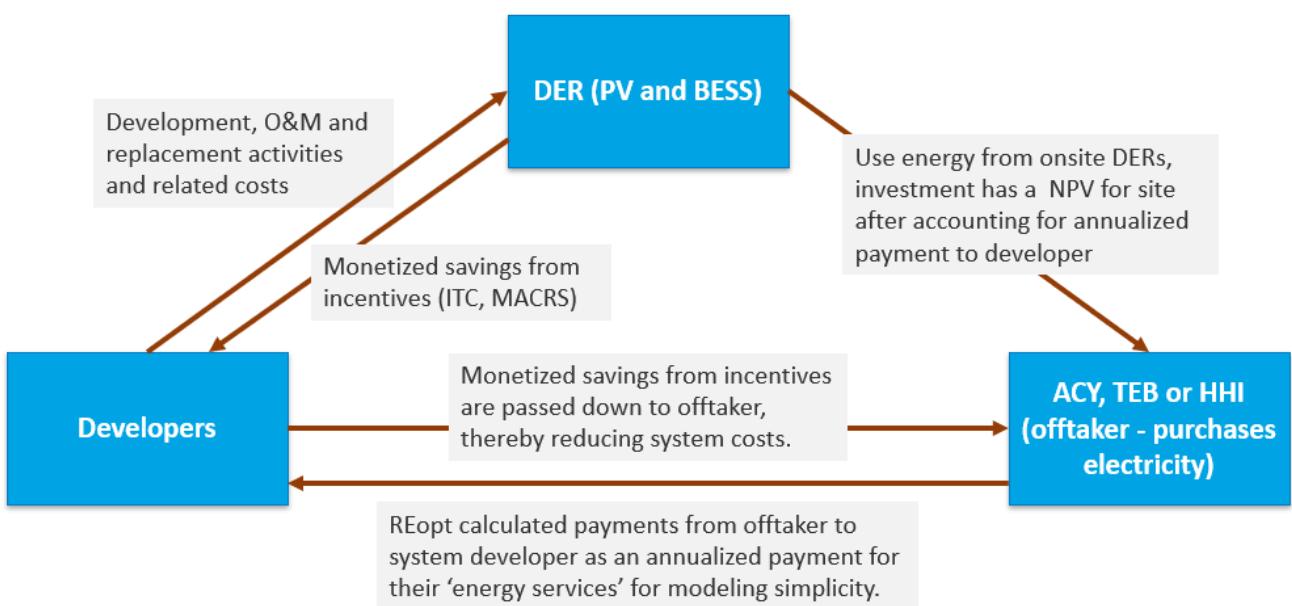
Figure 20. Third-party ownership model as implemented in REopt.
## 2.3.4 Technology Considerations
This analysis considers the following DERs to serve existing site loads plus eVTOL charging infrastructure at sites in the scope of the analysis. Technical details for each technology are described in Anderson et al. (2021).
## Solar PV
REopt considers south-facing standard rooftop PV with a 10° tilt angle and fixed axis. Each site’s corresponding coordinates were used to determine the solar resource from NREL’s National Solar Resource Database, which drives the energy production of a PV system. Solar PV is AC-coupled with the loads, which means all DC power output of PV gets converted to AC and takes a 4% efficiency hit in the conversion process. PV inverter clipping was modeled with a DC-AC ratio of 1.2. REopt default capital cost and operational cost values were used for PV. Due to third-party ownership of DERs, the PV system was modeled with a 30% ITC, 5-year MACRS, and 80% bonus depreciation, per updates from U.S. Congress (2022). These incentives are meant to come together to reduce the federal tax liability of the system developer. These assumptions and relevant data sources are described in Table 3. Per the latest FAA guidelines, airports are required to measure the impact of hazardous glint and glare from solar projects developed at airports on air traffic control operations and pilots (Federal Aviation Administration, DOT, 2021). This analysis does not consider the impact of glint and glare of any identified solar PV systems on airport operations.
Table 3. Solar PV Assumptions in REopt
| Input | Assumption |
| System type | Roof mount, fixed axis, standard module |
| Technology resource | Typical meteorological year (TMY) weather data from the National Solar Resource Database a |
| Inverter efficiency | 96% |
| Installed capacity density | 10 DC watts/ft² (O.01 kW/ft2); PV capacity that fits in roof top area |
| Tilt | Roof mount, 10° |
| Azimuth | 180°(south-facing) |
| DC-to-AC size ratio | 1.2 |
| System capital cost | $1,592/kW per 2022 NREL Annual Technology Baseline |
| O&M cost | $17/kW/year per NREL Annual Technology Baseline |
| Incentives b | 30%ITC |
| MACRS: 5-year depreciation with 80% bonus MACRS |
a https://pvwatts.nrel.gov/version\_6.php, https://nsrdb.nrel.gov/data-sets/tmy, https://sam.nrel.gov/weather-data.html
b REopt assumes all cost savings from incentives are passed through developer to system host.
## BESS
A lithium-ion BESS with 89.9% round-trip AC-AC efficiency was considered for the analysis. A battery’s performance can degrade if its state of charge drops too low (<10%) or if it is kept too high (>90%), making some battery capacity unusable. Therefore, REopt modeled the battery to hold at least 20% minimum state of charge to mathematically allow utilization of only 80% battery capacity. BESS capital cost was \$388/kWh, and cost of associated power electronics to charge and discharge the battery was \$775/kW. Because the performance of a battery degrades over its lifetime, REopt schedules a battery replacement in the 10th year of the analysis period where energy storage capacity costs \$220/kWh and power electronics cost \$440/kW. The replacement BESS is anticipated to last the remaining 15 years of the analysis period. The BESS is allowed to charge from the grid as well as any on-site PV. Additionally, BESS was modeled as eligible for 30% ITC and a 7-year MACRS depreciation schedule with no bonus depreciation, per updates from U.S. Congress (2022).
Table 4. BESS Assumptions in REopt
| Input | Assumption |
| Battery type | Lithium-ion |
| AC-AC round-trip efficiency | 89.9% (97.5% internal, 96% inverter, 96% rectifier) |
| Minimum state of charge | 20% (battery charge is managed to stay above this minimum) |
| Capital costs | $775/kW + $388/kWh based on Wood Mackenzie U.S. Energy Storage Monitor |
| Replacement costs (year 10) a | $440/kW + $220/kWh based on Wood Mackenzie U.S. Energy Storage Monitor |
| Allow the utility grid and any on-site PV Yes to charge the battery? | |
| Incentives b | 30% ITC |
| MACRS: 7-year depreciation with 0% bonus MACRS |
a Default one-time battery replacement occurs during year 10 of the analysis. REopt can also model replacement and augmentation battery replacement strategies.
b REopt assumes all cost savings from incentives are passed through developer to system host.
## 2.3.5 REopt Analysis Process and Scenarios
The process of analyzing site data and transforming them to usable REopt inputs is summarized in Figure 23.

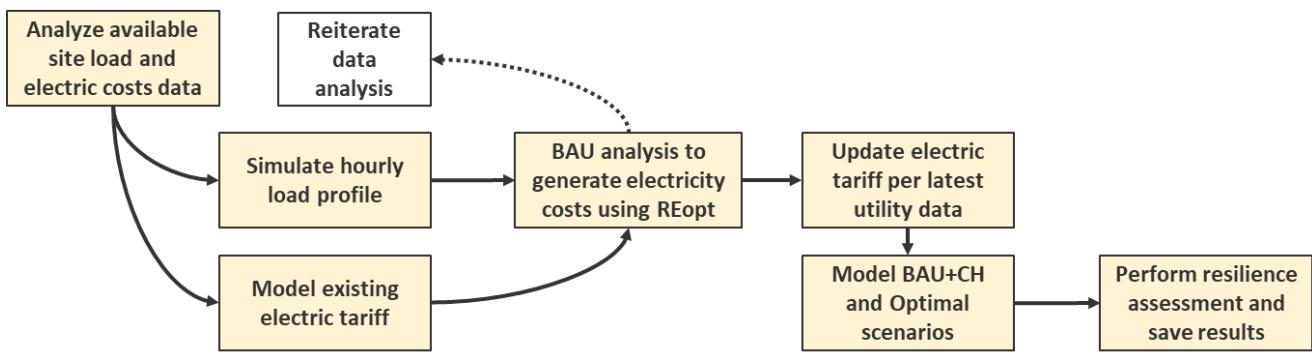
Figure 21. Steps taken as part of the REopt analysis for sites.
First, electricity costs and consumption data were collected from provided electric bills for analysis to determine the electric utilities and rate schedule servicing each site. Because hourly site operational load profile was unavailable for all three sites, DOE’s CRB load profiles were used to simulate the operational load profiles. Next, the following scenarios were executed for these sites, which are also summarized in Table 5:
BAU (Scenario 1): REopt was run using the simulated load profiles and electric tariff2 in an attempt to replicate the billed electricity consumption and costs in REopt. The purpose of this step is to validate the simulated load profile and electric tariff inputs and ensure no components are missing. This validation step is done by finding the percent difference between annual
electric bill costs per billing data and REopt results and reiterating over input data if the percent difference is higher than a certain threshold.
BAU With EVSE Charging (BAU+CH) (Scenario 2): This scenario considers the impact of EVSE load additions on utility costs. Results from this scenario quantify the implications of adding EVSE loads to site operational loads without any new on-site DER capacity.
Optimal (Scenario 3): This scenario considers the costs and benefits of including solar PV and BESS in conjunction with additional load of EVSE.
Optimal\_Restricted (Scenario 4): This is similar to the Optimal scenario (Scenario 3) but restricts the on-site solar PV size to rooftop area or existing solar PV system sizes.
Resilience: Results from Optimal and Optimal\_Restricted scenarios were used for resilience assessments for these sites. For HHI, the existing on-site generator was also included in the analysis to reflect the impact of on-site dispatchable DERs on resilience per assumptions described in Table 5.
Table 5. Summary of Scenarios Evaluated in REopt for Each Site
| # | Scenario | Purpose | Considers Existing Load | Considers EVSE Loads | Considers Cost-Optimal PV + BESS |
| 1BAU | | Site continues normal operations without any changes to its electric loads | | | |
| 2BAU+CH | Site adds eVTOL charging loads to its operational load profile and continues operations without any new DERs | √ | | |
| 3 | Optimal | Site adds eVTOL charging loads to its operational load profile and continues operations with an option of adding on-site solar PV, BESS | | 」 | |
| | 4 Optimal_restricted Site adds eVTOL charging loads to its operational load profile and continues operations with an option of adding on-site solar PV, BESS constrained by rooftop/land area restrictions | √ | | |
| 5 | Resilience runs | Assessing the resilience of cost- optimal systems to withstand a 4- hour outage | + | | |
## 2.3.6 Site Electric Load and Electric Tariff Summary
This section summarizes the electric tariffs (demand and energy charges) along with parameters used to synthesize the electric load profiles at sites. Due to the absence of interval data (or utilityprovided site-specific electric load data), a blend of DOE’s CRB load profiles was used to simulate site operational loads after reviewing services offered at sites via websites and Google Maps.3 This section also provides a breakdown of the proportion of various load profiles used for each site.
Teterboro Signature Flight Support Building (TEB)
• Electric utilities: Public Service Electric and Gas Company (PSE&G) and Talen Energy Marketing LLC
o Electricity generation service is provided by Talen. Because no rate plan information was available, average energy rates (\$/kWh) for each month were calculated and used for in inputs to REopt (Figure 24).
o Electricity distribution service is provided under PSE&G’s Large Power and Lighting – Secondary (LPLS) rate schedule (Table 6).
No interval data were available for TEB, so the load profile was simulated using the following “blend” of DOE CRB load profiles: 40% medium office and 10% warehouse. Additionally, 50% of the site’s load was modeled as flat load. Monthly consumption in kilowatt-hours extracted from billing data was used to scale up load profile appropriately.
Table 6. PSE&G LPLS Rate Schedule Breakdown
| Tariff | Charge | Applies To |
| Annual demand charge | $3.8176/kW | Monthly peak demand |
| Summer demand charge $9.0803/kW | | Highest demand measured during on-peak hours during summer months |
| Monthly customer charge $370.81 | | Per customer per month |
| Societal benefits | $0.010413/kWh Surcharge | |

Figure 22. Average energy prices used for TEB modeling.
ACY Terminal, Parking Garage, and Federal Inspection Station
• Electric utilities: Atlantic City Electric and Constellation Energy
o Electricity generation service is provided by Constellation Energy via its fixedrate plan. In the absence of appropriate energy rate information, this analysis utilizes monthly calculated energy rates (\$/kWh) for ACY (as shown in Figure 25 and Table 7).
o Electricity distribution service is provided by Atlantic City Electric’s Annual General Service – Secondary (AGS) rate, described in Table 8.
The load profile was simulated using the following “blend” of DOE CRB load profiles: 35% small office, 20% warehouse, 15% fast food restaurant. Additionally, 30% of site load was modeled as flat load. Monthly consumption (kWh) extracted from billing data was used to scale up load profile appropriately.
Table 7. Breakdown of Atlantic City Electric’s Annual General Service – Secondary (AGS) Rate Schedule
| Electric Tariff Component | Charge | Applies To |
| Fixed monthly charge | $193.22 | Per customer per month |
| Monthly transmission charge | $12.44/kW | Peak kW measured per month |
| Monthly distribution charge | $5.62/kW | Peak kW measured per month |
| Monthly demand surcharge | $0.278/kW | Peak kW measured per month |
Table 8. Breakdown of Energy Charges Used for ACY
| Electric Tariff Component | Charge | Applies To |
| Energy charges | See Figure 25 | All energy consumed on-site |
| Surcharges on energy consumption | $0.0224/kWh | All energy consumed on-site |

Figure 23. Average monthly energy prices for ACY per electric bills.
HHI
## Electric utilities: PSE&G
o Electricity generation service is provided by PSE&G’s Basic Generation Service, which relies on PSE&G-wide market rates for energy rates. Market rates from 2021 were used for HHI analysis and are shown in Figure 26.
o Electricity distribution service is provided by PSE&G’s General Light and Power, described in Table 9.
Note that once charging loads are added, the HHI site should get switched to the LPLS rate schedule, which is described in Table 6.
The combination proportions were informed by the facility functions per HHI’s website and through visual inspection of the site using Google Maps. The following building types were used in the blended load profile: 50% small office to capture the official work environment and pilot cafeteria and 20% as warehouse. Additionally, 30% of the site load was modeled as flat load to capture loads that may be constantly turned on. Monthly consumption (kWh) extracted from billing data was used to scale up load profile appropriately.
Table 9. Breakdown of General Light and Power Rate Schedule and BGS Energy (Utility Company) Charges Used for HHI
| Electric Tariff Component | t Charge | Applies To |
| Fixed monthly charge | $4.95 | Per month |
| Monthly demand charge | $3.9802/kW | Peak kW measured per month |
| Summer-only demand charge | $9.7113/kW | Peak kW measured in summer months |
| Distribution kWh charges | $0.007789/kWh October-May $0.003052/kWh June-September | Applies to all energy consumed on- site, but varies by month of year |
| Societal benefits charges | $0.009766/kWh | Applies to all energy consumed on- site |
| BGS energy charges | Real-time hourly varying energy charges | PJM Load Weighted Average Residual Metered Load Aggregate Locational Marginal Prices for the Public Service Transmission Zone |
| BGS energy charge adjustments | Adjusted for losses | Adjusted for hourly losses and adjusted to remove the mean hourly PJM marginal losses of 0.7164% |
| Ancillary service charges | $0.006/kWh | Applies to energy rates in all hours. This value also includes PJM's administrative charges and should be adjusted to hourly losses and mean hourly PJM losses of 0.7164%. |
| Monthly BGS capacity and transmission charges | $21.1552/kW summer/winter coincident peak | Meant for PSE&G to recover costs of operating and maintaining electricity generation services to service its area/zone |

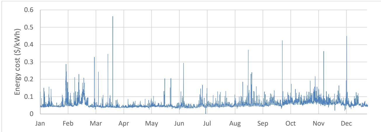
Figure 24. Plot of hourly energy charges used as HHI’s energy rate.
Two additional sites (HRHC and AtlantiCare), which were included earlier in the report, were not considered for a REopt analysis. HRHC’s existing power consumption is higher than the anticipated peak EVSE charging loads, which means grid impact would be minimal. AtlantiCare Hospital was not considered for REopt modeling because no EVSE chargers can be installed onsite due to it being a hospital.
## 2.4 Estimating Greenhouse Gas Emissions
The methodology for estimating GHG emissions resulting from total operational electricity consumption at the facilities included in this study adheres to the accounting framework provided in The GHG Protocol for Project Accounting (Greenhouse Gas Protocol 2005) and the supplemental guidelines provided in the Guidelines for Quantifying GHG Reductions from Grid-Connected Electricity Projects (Greenhouse Gas Protocol 2007). Key elements of this accounting framework include:
• Defining the boundary of the assessment
• Identifying a baseline scenario and estimating baseline emissions
• Identifying project scenarios and estimating the emissions for each.
The three primary GHGs included in this assessment are carbon dioxide (CO2), methane (CH4), and nitrous oxide $\left( \mathrm { N } _ { 2 } \mathrm { O } \right)$ , which are converted into a common reporting unit called “carbon dioxide equivalent” $\left( \mathrm { C O } _ { 2 } \mathrm { e } \right)$ using each gas’s global warming potential. As such, results will be reported in units of $\mathrm { C O } _ { 2 } \mathrm { e }$
## 2.4.1 Defining the Boundary of the GHG Assessment
The evaluation of GHG emissions for this study is limited to the facility electricity consumption at sites identified in Section 2.1.1 and selected for eVTOL assessment (ACY, TEB, and HHI). GHG emissions are estimated using electricity data provided by these sites and modeled for project scenarios along with location-specific emissions factors for grid-sourced electricity. To align with other model outputs and available emissions factor data, the temporal span of this GHG emissions analysis is 2024 through 2050, with calculations biennially from 2024–2030 and every 5 years from 2030–2050.
## 2.4.2 Analysis Scenarios
For continuity with other analysis completed by NREL, the outputs of the REopt models are used as inputs for the GHG emissions calculations. The scenarios described in Table 5 are also carried forward to the GHG emissions analysis.
## 2.4.2.1 Baseline Scenario
Quantifying a projection of the estimated change in GHG emissions from projects under consideration at these sites involves comparing the emissions modeled in project scenarios with a baseline scenario of what GHG emissions would be generated in the absence of project scenarios over the same time period (i.e., “business as usual”). As such, one of the most critical elements of the GHG emissions assessment is deriving a reasonable and accurate estimate of baseline emissions.
For this assessment, the baseline emissions scenario relies on three primary factors:
1. Historical metered electricity consumption at each site.
These data are used to determine the base year for the assessment at each site: ACY (2021), TEB (2021), and HHI (2021/2022).
2. Assumed load changes at each site over the 10-year assessment period (independent of load changes modeled in project scenarios).
FAA has advised NREL to assume zero organic load growth/decline over the assessment period.
3. Projected changes in the emissions intensity of the regional power grid surrounding the sites.
Annual emissions factors for grid electricity in New Jersey from the NREL 2022 Cambium data are used to estimate future emissions associated with electricity consumed from the power grid at the assessed FAA sites. These emissions factors are annual average values that represent the CO2e emissions resulting from power generation in a given geographic region during a given year.
## 2.4.2.2 Project Scenarios
This assessment evaluates projected GHG emissions resulting from three project scenarios in comparison with the baseline scenario:
Increased electricity demand for eVTOL aircraft charging loads at the identified sites, in alignment with outputs from BAU+CH from the REopt model.
Demand for grid electricity after the installation of cost-optimal on-site renewable energy generation system(s) that supply the electricity needs at each site, with the assumed increase in electrical charging demand in the BAU+CH scenario.
Demand for grid electricity after the installation of on-site renewable energy generation system(s) that meet the cost-optimal and site roof area constraints in the REopt model Optimal\_Restricted scenario (if applicable).
## 2.4.3 GHG Emissions Accounting Methods
Two different approaches to GHG emissions accounting are used in this analysis to express the way the project scenarios are estimated to influence GHG emissions: (1) attributional accounting and (2) consequential accounting. Both methods are widely accepted and useful in their own way, but it is important to note that they are not meant to be combined or compared.
## 2.4.3.1 Attributional Accounting
Attributional accounting of GHG emissions is used to assign ownership or responsibility to a given organization or entity for the emissions that are caused by their activities. This method is applied in the development of organizational GHG emissions inventories and can be used to express the emissions “footprint” associated with a certain activity.
To calculate emissions using this method, activity data (i.e., kilowatt-hours of electricity consumption) are gathered for a given time period and typically multiplied by an emissions factor associated with that activity (i.e., kilograms of CO2e per kilowatt-hour of grid electricity). To most accurately attribute the emissions to the entity being evaluated, the activity data must be actual measured data or reliable projections/forecasts of expected measured data in the future. In other words, the activity data are built “from the ground up” to account for the total level of activity carried out by the entity during the assessment period.
In this analysis, attributional accounting is used to estimate the GHG emissions that would be caused by electricity consumption at each of the included FAA sites from 2024 through 2050. These emissions would be attributable to (i.e., “owned by”) each site based on the amount of electricity consumed and the source(s) that supply that electricity. The calculation is simply:
## ???????? ???? ???????????????????????????? = ???????????????????????????????????????????? ???? ???? ???? ???? ???? ???? ∗ ???? ???????????????????????????? ???? ???? ????
The sources of electricity in this analysis include the regional power grid and on-site solar PV. While the emissions rate of solar PV is zero, the emissions rate of the regional power grid is dependent upon the mix of power plants that supply electricity to New Jersey and the surrounding area during a given period. For the baseline year of this analysis, the U.S. Environmental Protection Agency (EPA) Emissions & Generation Resource Integrated Database (eGRID) 2020 total output emissions factor for New Jersey was used in conjunction with the actual metered electricity consumption at each site. For the future years, the projected grid electricity emissions rates rely on various assumptions about the potential technology and policy development in the future. The NREL 2022 Cambium data (Gagnon, Cowiestoll, and Schwarz 2023) provide modeled forecasts of regional grid emissions rates under several scenarios. For this assessment’s calculation of GHG emissions using the attributional accounting approach, the annual average emissions rate for New Jersey under the mid-case scenario was used.
## 2.4.3.2 Consequential Accounting
Contrary to how attributional accounting of GHG emissions assigns ownership of/responsibility for emissions to a given entity and builds a “footprint” out of actual activity data, the consequential accounting method is used to evaluate the emissions that would be caused or avoided by a particular change in activity without attributing the emissions to any one entity. This method is often used to evaluate hypothetical scenarios in comparison with a counterfactual scenario in which the decision/action being evaluated does not occur.
The calculation of emissions uses the same general formula as the one used in attributional accounting; however, the input data are different in the consequential accounting method. The activity data is the change in activity and the emissions rate is specific to the change in activity. For this assessment of GHG emissions related to electricity consumption, the marginal change in electricity consumption in each scenario must be multiplied by a specific marginal emissions rate.
Because the project scenarios that are assessed involve changes to the FAA sites’ loads, marginal emissions rates are applied to the incremental change in electricity consumption to calculate the estimated change in GHG emissions compared to the baseline scenarios. Marginal emissions factors differ from annual average emissions factors in that they represent the emissions generated by power plants that are forced to operate in response to marginal changes in demand on the power grid. These power plants are typically less economical, less efficient, and more polluting than other power plants and are therefore dispatched by power grid operators only
when needed. These emissions rates are also referred to as “short-run marginal emissions rates” (SRMERs) because the grid is responding to marginal load changes it has not planned for.
Alternatively, long-run marginal emissions rates (LRMERs) can be used to analyze the emissions resulting from sustained long-term changes in electricity demand (e.g., projects that increase site power loads, energy efficiency projects, on-site power generation) that result in structural changes to the power grid. In other terms, the LRMER represents a marginal emissions factor for a future in which the grid has built new capacity (or some other structural intervention) in response to the long-term change in demand.
The NREL Cambium data sets contain modeled SRMERs and LRMERs for a range of possible futures of the U.S. electricity sector through 2050. This analysis utilizes mid-case scenarios for both SRMERs and LRMERs to estimate future emissions changes in the project scenarios. In alignment with recommended uses of SRMERs and LRMERs by NREL Cambium authors, this analysis for FAA assumes SRMERs for 2024–2028 and LRMERs for 2030–2050.
## 2.5 Hazards and Risk Analysis
## 2.5.1 Electric Vehicle Supply Equipment Hazards
EVSE infrastructure faces natural, human, and technological hazards—with significant overlap between each in many scenarios. Natural hazards derive from climate- and weather-induced events or seismic activity. Human hazards may be unintentional errors or intentional attacks to critical infrastructure. Technological hazards are most easily understood when delineating the effects of human or natural hazards between the electrical distribution system and the energy storage system.
Natural hazards vary between locations due to topology and geographic location. Unlike climaterelated hazards, seismic risks must be addressed through the National Electrical Code for any relevant equipment or structures. Warm and humid coastal regions are more prone to flooding, hurricanes, and tropical storms, unlike other regions that experience yearly snowfall at higher altitudes, and also can vary from regions with high tornado incidences or seismic activity. Coastal regions must also consider saltwater corrosion, water table location for any underground structures, and high-strength winds on aboveground electrical infrastructure. Regions with high tornado activity, often not the same regions with high tropical storm activity, must also consider infrastructure reinforcements to survive high winds. Regions with extreme temperatures must comply with the manufacturer-suggested operating conditions to achieve optimal performance. Severely cold conditions may decrease battery discharge rates and in turn alter vertiport operations or aircraft scheduling. Snow removal, either with heavy equipment or MgCl for deicing, also poses collision, corrosion, and fire risks if any unintentional operator errors occur.
Human hazards must be mitigated in ways that minimize harm to the electrical infrastructure as well as the operating personnel. As in the case of snow clearing or de-icing in colder climates, a human hazard can be operator error of heavy equipment when removing snow, eVTOL operations, or the potential electrocution or arc flash associated with the damaged electrical equipment. In severe cases, fires and explosions can occur when electrical equipment is damaged. Thus, human hazards exist alone or in tandem with natural hazards that need to be alleviated.
When identifying technological hazards, most risk is inherently present with the equipment in place and can be heightened as an effect of natural or human hazards. The transformers, conductors, connectors, and other equipment associated with the distribution system and charging equipment all have electrical hazards—shock, arc flash, electrocution, and fire—that are present all the time. Faults or damage to the system can be induced by an outside agent (natural or human hazards) or degradation over time. In both situations, the risks and their severity must be mitigated to avoid cascading system damage and/or harm to the operating personnel. A battery storage system poses electrical, thermal, and chemical hazards of its own. Battery management systems can monitor the risk of overcharging/discharging, thermal runaway, overheating, and electrode destabilization. In the case that there are catastrophic events occurring in or around a BESS, many National Fire Protection Association regulations provide guidelines for handling and suppressing any fire or explosive hazards. Additional details are provided in the separate report including hazards associated with eVTOL charging infrastructure by Rane et al (2023).
## 2.5.2 Cybersecurity Evaluation
Associated with intentional human hazards, the risk of cyberattacks on critical electrical infrastructure is brought about by physical means or by remotely deploying malicious malware that results in hindered or terminated operations. These types of attacks can affect not only the charging infrastructure at the site, but also the aircraft and local grid if the control system or charging connectors are compromised. Thus, supply chain and network access management are key focal points to provide holistic charging infrastructure protection. For example, the EVSE communications network at the site between charging infrastructure and central controllers is often interconnected through Open Charge Point Protocol, and if not implemented securely, various attack angles are left vulnerable (Markel and Sanghvi 2022). With significant overlap with vehicle charging systems, many of the lessons learned and best practices should continue to be implemented in the aviation industry to achieve seamless, integral, and functional cybersecurity.
## 2.6 Estimating Economic and Job Impacts
For this modeling work, the required charging infrastructure for eVTOL aircraft in New Jersey and New York is expected to create local jobs in multiple sectors, as well as stimulate the local economy of both states. To estimate the economic impacts of these ground infrastructure projects, we use an input–output (IO) model, one of the most commonly used and straightforward methods for estimating economywide impacts due to a change in regional demand (e.g., a new construction project). IO models are composed of several equations reflecting each sector’s production function (i.e., their production “recipes”) that together show how these sectors interact in a region. This is accomplished by modeling the structure of an economy as a network of sectors buying and selling to one another, local households, government, and external markets. Its results reflect the supply chain’s responses and the total macro-level impacts from changes in demand for goods or services in a region.
IO models capture “multiplier effects” in the economy that arise from sectoral interaction across different supply chains. A change in demand acts as a drop of water in a still pond creating waves (“ripples”) that are large in the beginning and fade over time. The first wave is the largest: It represents the change in the purchasing pattern of directly affected firms. To meet the demand for goods and services of this first wave, suppliers of these firms need to change their purchasing patterns, generating a secondary smaller ripple. Then, suppliers of these suppliers also need to change their purchasing patterns, and so on, generating a sequence of fading ripples in the economy. The sum of all ripple effects is the total economic impact of that initial change in demand.
A few examples of IO analysis in energy-related projects are Jeffers et al. (2022), who used the IO framework to estimate the economic effects of the deployment of zero-emission buses (battery electric and fuel cell) and related infrastructure in California; Navigant (2020), who estimated the impacts of a replacement project for Astoria Gas Turbine Power in New York state; and Lahr, Coughlin, and Felder (2010), who analyzed the statewide impacts of natural gas infrastructure projects and residential solar lease programs in New Jersey.
## 2.6.1 Approach and Data
Construction and operation costs from different charging infrastructure projects will be separated by state to estimate temporary and permanent economic effects. From the total amount of investments in a region, part of the goods and services are provided by companies outside the state (nonlocal purchases) and do not generate local impacts (Figure 27). Those are excluded from the analysis using state-specific regional purchase coefficients that determine the percentage of local purchases for each good/service in the model (these vary by year due to the evolving regional economic structure). The amount of local purchases is then used to introduce a demand shock in the model and to determine the total economic impact including jobs created in each state due to these investments.

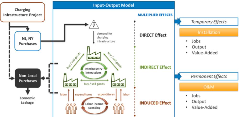
Figure 25. Economic impact analysis overview.
Impacts can be classified as direct (immediate economic impact from the change in demand), indirect (from supply chain linkages), or induced (resulting from the spending of wages/salaries by workers) by region. The results include total temporary and permanent jobs created, changes in gross regional product (value added), and sectoral output:
• Jobs are defined as the sum of full-time and part-time workers (measured in full-timeequivalent jobs) employed at the place of business. All jobs supported by local companies are accounted for, including those of out-of-state commuters (who might spend part of their wages outside the state).
• Output represents the value of production and includes all sales and purchases of a particular sector.
Value added represents the wealth generated by an economic activity and includes compensation of employees (wages and benefits), profit-type income, property income, and taxes on production.
Gross regional product measures the monetary value of final goods and services produced in a region and is the sum of all sectors’ value added.
For this analysis we used IO data from the U.S. Environmentally-Extended Input-Output (USEEIO) project (EPA 2023a). USEEIO is a publicly available platform developed and maintained by the EPA that provides IO tables connected to a series of socioeconomic, environmental, and resource use metrics (EPA 2023b). Its stateior (EPA 2023a) extension provides data for each U.S. state at the U.S. Bureau of Economic Analysis Summary Level (71- sector disaggregation) for 2012–2020. From this data set, we used the 2019 multiregional IO table for New Jersey, which has two interconnected regions: New Jersey and the rest of the United States. Data for 2020 were not considered due to the transient effects of the COVID-19 pandemic on the economic structure of these states.
Infrastructure data for each site were obtained from the previous analyses and represent installed costs in purchasing prices (i.e., include transportation and wholesale/retail margins). Each itemized expense was broken down into direct costs (labor, materials, equipment rental, and subcontract), indirect costs (construction management, engineering, startup, and permitting), and contingency costs according to the assumptions used in Burns and McDonnell (2019) and shown in Table 10. Next, each cost was allocated to an economic sector in the model according to the Bureau of Economic Analysis summary-level disaggregation. Costs were deflated to 2012 prices, and purchasing values were separated into producer costs, transportation costs, and wholesale/retail margins using the 2012 Benchmark Input-Output Margins table (BEA 2018). Finally, the adjusted costs were deflated to 2019 prices to match the year of the USEEIO IO tables.
Table 10. Expense Allocation Assumptions
| Expense | Cost Allocation | Sector Allocation |
| Direct |
| Labor | Based on equipment specific data from Burns and McDonnell (2019). Labor rates were adjusted to reflect New | 2332D0b |
| Materials | Material-specific |
| Subcontract | Material-specific |
| Equipment rental | 532400c |
| Indirect |
| Construction management 15% of direct costs | | 2332D0 |
| Engineering | 12% of direct costs | 541300 d |
| Startup | 6% of direct costs | 2332D0 |
| Permiting | 2% of direct costs | GSLGOe |
| Other |
| Contingency | 25% of direct + indirect costs | 2332D0 |
| Contractor | 5% of direct + indirect costs | 2332D0 |
a Labor rate was adjusted using state wage data for 2021 from the Bureau of Labor Statistics’ Occupational Employment and Wage Statistics (https://www.bls.gov/oes/).
b Other nonresidential structures.
c Commercial and industrial machinery and equipment rental and leasing.
d Architectural, engineering, and related services.
e State and local government (other services).
Total infrastructure costs per site are shown in Figure 28. Total charging investment is the same for all sites, \$1.4 million (2021 prices). For this analysis, we allocated the Feeder A grid investment to ACY and the Feeder B investment to HRHC. Because of the model aggregation (state level), this assumption will not impact the results of Feeder B.

Figure 26. Total investment by site and category.
O&M data for each site were estimated according to Table 11 assumptions. Charging infrastructure O&M annual cost is based on a 325-kW charger’s maintenance costs from Burns and McDonnell (2019), and its breakdown was based on Jeffers et al. (2022). O&M annual cost for microgrid and grid infrastructure was based on NREL’s Jobs and Economic Development Impact (JEDI) Transmission Line Model (rel. TL12.23.16) (NREL 2023d) and depends on both total capital investment and transmission line length. These data were allocated to different economic sectors and adjusted in the same way as the infrastructure data.
Table 11. O&M Yearly Cost Assumptions
| Expense | Assumptions | Sector Allocation |
| Charging Infrastructure | | |
| Labor/personnel | $1,963/chargera V001 | |
| Insurance | $1,950/charger a 5241XX | |
| Replacement parts/equipment/spare parts $ | | $2,499/charger a Material-specific |
| Licensing and permits | $195/charger a | GSLGO |
| Overhead | $393/charger a | 230301 |
| Substation/Converter Station Infrastructure | | |
| Labor/personnel | 0.1% of TCI b | V001 |
| Insurance | 0.2% of TCI b | 5241XX |
| Replacement parts/equipment/spare parts 0.1% of TCI b | | Material-specific |
| Transmission Infrastructure | | |
| Labor/personnel | $8,193/mib | V001 |
| Maintenance materials | $2,028/mib | 335999 |
| Insurance | $1,155/mi b | 5241XX |
| Replacement parts/equipment/spare parts $1,240/mi b | | Material-specific |
a Based on Burns and McDonnell (2019) and Jeffers et al. (2022); assumes an annual maintenance cost of \$7,000/yr per 350-kW charger.
b Based on JEDI Transmission Line Model (rel. TL12.23.16); TCI = total capital investment.
Total annual O&M costs per site are shown in Figure 29. Annual charging costs are the same for all sites at \$28,000/yr (2021 prices). Similar to infrastructure costs, Feeder A O&M costs for the combined is allocated to ACY, and Feeder B O&M costs are allocated to HRHC, but the latter results apply to both sites.

Figure 27. Annual O&M costs by site and category.
## 3 Results
## 3.1 Vertiport Electrical Infrastructure Upgrade Needs
eVTOL OEMs reported peak DC charging loads of 300 kW to 1 MW. A lesson learned from EVSE deployment for light-duty vehicles was that more power capacity was needed to meet charging speed demands for newer vehicles purchased by consumers. NREL recommends vertiports plan for 1 MW (and potentially higher) to align market speed of deployment with utility upgrade timelines. Potential demonstration or permanent sites should engage early with the utility on site selection, as they can indicate if a potential site may result in higher or lower costs for adding capacity and infrastructure. A significant factor for site cost is the distance between the electrical panel and charger—greater distances usually include more construction, trenching, and digging to bring power to the location. Where possible, site the vertiport close to existing transformers and ideally use three-phase power.
For stationary chargers, eVTOL aircraft can either be charged at the vertiport landing area or moved to a nearby charger. This largely depends on the eVTOL aircraft configuration; those with wheels could taxi to a charger or be moved by tractor, tug, or tow vehicle. eVTOL aircraft with skids can be moved by attaching ground handling wheels via a hydraulic or cam mechanism. Another option is a tow cart—an electric or hydraulic device that attaches to the eVTOL skids, where it can be driven to the EVSE.
Mobile charging is also a consideration. For reference, a recent demonstration of mobile charging for light-duty vehicles found that it is not currently economically competitive. The 80- kWh unit takes approximately 10 hours to charge and costs 4–5 times more than stationary chargers. While mobile charging with batteries affixed on a truck is feasible for ground-based vertiports, more challenges are anticipated for rooftop locations. Considerations for mobile charging on a garage rooftop vertiport include the height and weight restrictions for mobile charging vehicles, as well as turning radius to reach the rooftop. Assuming there is sufficient room on the rooftop to accommodate a charging truck outside the safety zone, another consideration is how to secure access to the site for a charging vehicle. One potential avenue for study is the feasibility of mobile trucks on the ground level supplying charging cables that are installed on the roof to provide more options and flexibility for charging, thus reducing limitations on rooftop access.
There are currently limited charging infrastructure cost estimates available for eVTOL aircraft, and the numerous EVSE hardware manufacturers result in a range of costs. The more significant costs are installation and utility service upgrades, which will vary widely based on utility upgrades needed, distance of EVSE from the power source, amount of trenching needed, and whether equipment needs to go under a highway, runway, or other significant infrastructure. There are also many soft costs such as complying with Americans with Disabilities Act (ADA) requirements, which can impact overall costs.
As one example, a NASA-funded study estimated \$883,000 for a single rooftop charger on a five-story building at an existing landing site (Black & Veatch 2019). The estimated cost for three landing pad sites and a pod with three chargers was \$2,630,000 (see report for details on what is included in these costs). The assumption for the chargers is 600 kW, 480 V, and 800 A.
The ground charging assumes space of 500 ft by 170 ft and inclusion of a prefabricated waiting area. It was also assumed the utility would provide a new feeder, and utility costs are not included in these estimates. The report assumed a timeline of 9–12 months for permitting and buildout for both scenarios, which could be aggressive.
Infrastructure costs for high-voltage charging equipment dedicated to aviation are not readily available. A potential proxy for infrastructure costs are limited data for transit bus en route fast charging. Based on data obtained from a survey of transit agencies, the average cost of a highspeed charger is \$495,636 (range of \$330,000–\$600,000) (NASEM 2018). An NREL transit bus analysis assumed a peak draw of 325 kW per charger (Johnson 2020). Significant future cost data for 350-kW chargers are expected from stations funded by the Joint Office of Energy and Transportation, which could help inform cost ranges for eVTOL charging.
Charging demand to support electrified aviation needs can range from kilowatts to megawatts, which can impact the existing utility grid infrastructure; thus, it is important to include the local public utility as a key stakeholder during the planning/conceptual design phase to prevent avoidable costs and delays in project implementation.
The utility is expected to be primarily interested in understanding the power capacity, number of charging stations, and any potential future expansion from the electrification point of view. In most cases, the meter owner (site host) needs to identify the charging infrastructure details, with the utility focused upon servicing that electrical demand without affecting power quality for the serving areas. For larger sites (such as a public use airport) that utilize utility-serviced distribution and facility metering, potentially hundreds of meters converge. Airports are currently looking to accommodate changes in electrical demand from ground vehicles and thermal loads in addition to aircraft loads. Airport sponsors may wish to consider longer-term installation energy planning to assist with regional utility planning with energy resilience goals based on the overall facility’s requirements.
Based on the projected electrical demand information, the utility may carry out various studies including power flow analysis to analyze the impact on the existing off-site infrastructure and to identify if any infrastructure upgrades are required to accommodate the future on-site demand. The infrastructure upgrades may include, but are not limited to, transformers, distribution lines, voltage regulators, and/or protection equipment. The time necessary for infrastructure upgrades for significant requests (utility planning, installation, and commissioning) can take up to 4 years depending on the upgrades required (Borlaug et al. 2021). It is noted for initial adopters, utility services when initially installed are typically sized for theoretical peak demands, such that once they are in service they may allow for incremental load increases on the transformer without this significant infrastructure upgrade process.
In order to engage with the utility, the site host needs to identify what EVSE infrastructure is needed to meet the potential vehicle charging demand. NREL has developed various tools including EVI-EnSite, which can be used to study operation and quality of service of charging station configurations from low power to high power and determine the charging demand for different scenarios (NREL 2023b). Demand includes both potential peak requirements and quantity of energy needed, ideally including load profiles through a typical recurring period of time (day, week, or year). These data are also helpful for site owners to determine behind-themeter management strategies to complement grid utility operations and manage cost of power delivered. In the absence of a detailed load profile, peak demand requirements will be utilized for necessary utility infrastructure sizing, providing a more robust facility sizing and associated capital cost.
Once the charging demand is determined, a utility-led load study may be conducted to identify the potential impact on the existing utility-owned electrical infrastructure. This study generally identifies any upgrades required in the grid electrical infrastructure avoiding any impact on power quality for the utility serving area and may require funding from the site owner. NREL has developed various open-source tools including DISCO, which can be used to study the impact of DER and load changes on distribution systems (NREL 2019). This tool provides key details from the study including loading status of various equipment and distribution lines, the various connection points of feeder with under- or overvoltage conditions, and potential solutions to mitigate the issues by voltage regulators and/or upgrading the infrastructure.
The site host also has an option to minimize the impact on the electrical infrastructure with onsite generation and energy storage solutions. To identify these solutions, the techno-economic analysis can be carried out considering financial and technical parameters of the DERs and associated accessories. NREL has developed the open-source Renewable Energy Optimization (REopt) tool to perform techno-economic analysis to identify the optimal mix of renewable energy, conventional generation, energy storage technologies, and electric vehicle charging to meet cost savings, resiliency, emissions reduction, and energy performance goals (NREL 2023e).
The U.S. Department of Transportation has provided a project planning checklist for EV infrastructure that is substantially relevant for eVTOL charging infrastructure. The checklist consists of four key states of the project and important tasks/information for those states, highlighting engagement with the utility and different ownership models for grid and charging infrastructure (U.S. Department of Transportation 2023). These ownership models are explained with some modifications, as well as adding the microgrid infrastructure for the ownership arrangements. There is a similar toolkit available for electric vehicles from the Federal Energy Management Program covering all the different steps and respective needed material (FEMP 2023). The toolkit includes key details such as electrification checklist, training material, planning and deploying of EVSE, and a utility finder. NREL has reported considerations about electric vehicles and charging infrastructure for the U.S. Department of Defense that can also be applicable for eVTOL charging infrastructure (Hodge et al. 2022). DOE has also provided different steps for charging infrastructure procurement and installation that detail considerations about costs associated with equipment, installation, and networking, as well as other considerations for including compliance, permitting and inspection, ownership, and utility participation (Alternative Fuels Data Center 2023).

Figure 28. Ownership models for different infrastructure.
Figure 30 presents the possible ownership scenarios between a utility, site host, or third party.
In the traditional approach, the utility is responsible for all the electrical infrastructure up to the utility metering connection, while from the metering point onward the site host is responsible for all the cost including owning, operating, and maintaining all the electrical, EVSE, and microgrid infrastructure. Note that the site host can work with different third parties for owning, operating, and maintaining any or all of the infrastructure including electrical, EVSE, and microgrid components with multiple financial arrangements for procurement and maintenance possible.
In the “Make Ready” approach, all the electrical infrastructure up to the connection of EVSE and/or microgrid would be managed by the utility for owning, operating, and maintaining. The site host will not have any upfront investment costs for the electrical infrastructure and related upgrades; the utility will recover or absorb these costs. The site host can work with the third parties for EVSE and microgrid infrastructure for installing, operating, and maintaining with multiple financial arrangements for procurement and maintenance possible. In the EVSE-only model, site electrical infrastructure remains with the site owner, while the utility will install, operate, and maintain EVSE and associated infrastructure occurring prior to the site meter. This could be a low-cost option if there is little or no upgrade required for on-site electrical infrastructure. An additional load could be desired in the future within the meter service area, along with any related backup power or microgrid systems supporting the charging systems. Similar to other alternatives, the site host can work with the third parties to install, operate, and maintain associated systems.
Should the site owner wish to pair energy generation assets with customer-owned EVSE in a manner that allows the system to operate in grid-connected and grid-independent mode (microgrid), the utility could be requested to install, operate, and maintain the microgrid along with electrical infrastructure until the metering connection. Note that the site host will still be responsible for the on-site electrical infrastructure upgrades and microgrid, and can work with the third parties for associated systems.
In the “EVSE and Microgrid Only” model, the utility could be requested to install, operate, and maintain EVSE and microgrid assets, along with electrical infrastructure, until the metering connection. Note that the site host will still be responsible for the on-site electrical infrastructure upgrades and can work with third parties for installing, operating, and maintaining with set financial mechanisms.
In the “Full Ownership” model, the utility would own, operate, and maintain all the infrastructure including the EVSE and microgrid. The utility would charge the site host for EVSE and generation from the microgrid.
Note that the utility can play a key role taking into account the potential incentives, discussing the demand charges applicable, and considering charging load, optimal charging strategy, and the business case of deferring the capacity expansion by on-site renewable generation and energy storage system. Also, each utility and regulation from the state may vary for sharing/applying costs associated with utility infrastructure upgrade with the site host. It is also noted that in many jurisdictions, the utility provider operates energy delivery under a regulated exclusive use agreement, while EVSE and energy generation services may operate under separate related entities that can operate on a for-profit basis.
Ownership and electrical infrastructure procurement and operations models will vary based upon specific jurisdictions and whether the proposed infrastructure is being installed on federally obligated facilities. Multiple scenarios discussed assume that proposed siting is compliant with site requirements and relevant procurement code. Many of the scenarios discussed provide various components of charging as a service, either from the utility, a third-party-financed scenario, or owned and operated by the site operator. Each case will vary in how the cost of energy delivered is recovered, both in capital and operational expenditures. The ownership/procurement models can vary based upon local utility rates and other considerations.
For federally obligated facilities, potential procurement models should be reviewed for airport compatibility. Examples of areas to explore during site electrical infrastructure planning include site availability, intended users (e.g., exclusive, nonexclusive use), utility easement opportunities, cost recovery models for airport operations, highest and best use for facilities, airport cost recovery models, existing fixed-base operator agreements, etc. Details regarding these additional requirements are beyond the scope of this effort, and relevant FAA and local guidance should be evaluated when considering alternatives to service this emerging market.
## 3.2 eVTOL Aircraft Charging Demand
To properly size energy systems for cost-optimal installation, estimating the realistic peak and overall energy demand for proposed operations is a crucial step. Daily or monthly loads do not reflect the technical charging dynamics or the demand charges that may be applied to very large peak loads in many cases. The following methodology was utilized to estimate energy demand for studied use cases.
As flights are scheduled, the aircraft operating conditions for the set route are referenced in the model to provide the energy demand for the specific route, aircraft, and number of passengers on the flight. The energy consumption for each route, vehicle, and number of passengers was calculated using the model outlined in Section 2.1. The energy consumption is unique to the aircraft’s configuration, which informs the aircraft battery’s expected state of charge at the destination vertiport. Figure 31 provides the expected range of average energy consumption for considered aircrafts on different routes with a range of passengers. Note that there is a notable difference in the energy consumption across routes and number of passengers. The average impact of a passenger is an increase of 5.5% energy consumption. The resulting state of charge and anticipated arrival time is then shared with the destination vertiport, and the aircraft is added to the inventory at that location.

Figure 29. Average energy consumed by aircrafts for different routes with different numbers of passengers.
Unlike on-road vehicles, eVTOL aircraft cannot charge along the route. Therefore, the model will not allow a flight to be scheduled until the aircraft is charged enough to reach the final destination, thus incentivizing fast charging and the availability of larger fleets at each location. In addition, there must also be a balance within the available fleet to achieve the most efficient use of each aircraft type.
As an initial condition, aircraft are assigned to each vertiport based on available space, and no eVTOL aircraft are parked at helipads at hospitals. TSS and PEG are in Manhattan and are more space-constrained than vertiports in New Jersey. Assumptions were also made about the number of chargers and power level. For the unconstrained scenario, unlimited 1-MW chargers are available at each vertiport except AtlantiCare Medical Center. For the constrained scenario, a maximum of three 300-kW chargers are considered (Table 12). Figure 32 and Figure 33 show examples of areas specified for seven parking spots and takeoff and landing areas at ACY and HRHC, respectively.

Figure 30. Example eVTOL parking and takeoff and landing area at ACY.

Figure 31. Example eVTOL parking and takeoff and landing area at HRHC.
Table 12. Vertiports Considered in the Simulation
| Vertiport | Number of Assigned Aircraft | Number of Chargers |
| ACY Atlantic City International Airport 7 | | 3 |
| HRHC Hard Rock Hotel & Casino | 7 | 3 |
| ACMC AtlantiCare Medical Center | 0 | 0 |
| ACAC AtlantiCare Atlantic City | 0 | 0 |
| HHI | HHI heliport | 7 | 3 |
| TEB | Teterboro Airport | 7 | 3 |
| TSS | TSS heliport | 3 | 2 |
| PEG | PEG heliport | 3 | 2 |
Passenger demand schedules were randomly generated using assumed weights for origin/destination, party size, and hour of day. This is important not only in the case of commercial airline passengers, but also because a significant portion of early adoption markets are targeting commuter-based travel in congested areas in large cities. Figure 34(a) shows the assigned weight for origin/destination, Figure 34(b) presents the assigned weight for origin and party size, and Figure 34(c) depicts the assigned weight for hour of the day the request was made at the origin. The highest weights were applied for the route between ACY and HRHC assuming the higher traffic for hotel and casino in Atlantic City to and from airport, party size of 3–4 for origin at AtlantiCare Atlantic City and AtlantiCare Medical Center taking into account the patient and emergency medical technician or nurses, and request times from 3–8 p.m., which can be typical peak traffic hours. The lowest weights were applied for the route between AtlantiCare
Atlantic City and AtlantiCare Medical Center considering use case for emergency only; party sizes of 5–6 for origin at AtlantiCare Atlantic City, AtlantiCare Medical Center, HHI, PEG, and TSS assuming use case for replacing the helicopter traffic; and request times after midnight and other late-night hours, which can be typical.

(a)

(b)

(c)
Figure 32. Likelihood/weight assigned for (a) origin/destination, (b) party size at different origins, and (c) time of request at different origins.
The distributions shown in Figure 34 are used to generate a schedule of passenger demand by first sampling from the origin-destination likelihood distribution to get the origin and destination of the trip, then using the trip origin to sample from the party size and time-of-day distributions. Each passenger is assigned a random name to make them easier to track, and some noise (±30 min) is added to their request time. For illustration, selected rows from the passenger demand schedule are shown in Table 13. The schedule includes origin, destination, time of request, and passenger details.
Table 13. Example Passenger Demand Schedule
| | Origin Destination Time of Request Passenger Details | |
| TEB | PEG | 1/1/21 0:12 | Claire A. |
| TEB | PEG | 1/1/21 0:12 | Jon J. |
| TEB | PEG | 1/1/21 0:12 | Ron R. |
| TEB | PEG | 1/1/21 0:12 | Melody J. |
| ACY | HRHC | 1/1/21 0:47 | Emanuel W. |
| ACY | HRHC | 1/1/21 0:47 | Wilson P. |
| ACY | HRHC | 1/1/21 0:47 | Markus N. |
| ACY | HRHC | 1/1/21 0:47 | Tameka K. |
Charging was carried out on a first-come, first-served basis at each vertiport at a constant power until maximum state of charge (100%) is reached. Note that the simplest realistic assumption to make would be constant (max) power from 0% to 80% state of charge, then a linear decay in charging power from 80% to 100%. The agent-based flight scheduling model optimization problem seeks to minimize passenger wait time and charging energy consumption at each site, considering one flight or less per origin vertiport per minute, one flight or less per route per minute, vehicle availability, and stored energy. The solver selects one flight for each vertiport and route to maximize global benefit. Flights are scheduled dynamically in response to passenger demand. A flight is defined by aircraft, passengers, route, takeoff time, and landing time. Bottlenecks at the vertiport mean longer wait times for passengers, and the number of passengers the system can accommodate is limited by number of aircraft (and seats), chargers (number and power level), and logistics (vertiports can run out of vehicles). For very high passenger demand, wait times grow exponentially (Figure 35). Due to limited charging stations at the sites, vehicle airborne time saturates at around 30% for the constrained scenario compared to the unconstrainted scenario (Figure 36). Considering these figures, reasonable use cases are around 1,400 passengers/day for the scenarios.

Figure 33. Wait times for passenger demand for both constrained and unconstrainted charging stations.

Figure 34. Vehicle airborne time achieved for passenger demand for both constrained and unconstrainted charging stations.
In terms of number of passengers (approximately 1,400) and charging, the simulation results show a maximum charging rate of 900 kW in the constrained case and 13.3 MW in the unconstrained case at ACY at 21:58 (Figure 37). Using ACY as an example, energy consumption is 34 MWh/day in the unconstrained case and 33 MWh/day in the constrained case, as shown in Figure 38 and Figure 39, respectively.

time
Figure 35. Charging demand profile for ACY with constrained and unconstrained charging station scenarios.

Figure 36. Energy dispensed for charging at different sites for unconstrained charging stations.
constrained, 5 trips/day/vehicle

Figure 37. Energy dispensed for charging at different sites for constrained charging stations.
Charging demands for constrained scenarios for ACY, HHI, HRHC, and TEB were applied to perform various studies, and their results are presented in the following sections.
## 3.3 Electrical Grid Impacts
A peak load day was selected for each feeder considering the overall feeder demand. Because the electrical grid becomes stressed with higher demand, the maximum load day was selected to evaluate the impacts of the worst-case scenario on the grid with added eVTOL charging demand. Power flow simulations were conducted for the peak day with 1-minute time step resolution under the three scenarios. This section presents the grid impact analysis results on feeders for the four major sites: TEB, ACY, HRHC, and HHI. First, the comparative analysis is presented for BAU (labeled Scenario 1, or “s1,” throughout the figures) and BAU+CH (labeled Scenario 2, or “s2,” throughout the figures), followed by the necessary infrastructure upgrade analysis results. Finally, the optimal scenario with energy storage is evaluated. It is important to note that the
actual size (capacity) of the transformers at the sites was not available, so the capacities of the transformers at the selected locations on the synthetic feeders represent the size of the real site transformers. The locations were chosen so that the existing transformers were enough to supply the present electrical demand of the actual sites, as identified in Section 2.1.3.
## 3.3.1 Analysis of the Feeders with ACY and HRHC
As discussed in Section 2.1.4, two test feeders were selected from those that supply the large airport in Austin. One of the feeders constitutes a larger part of the ACY load, and the second includes the remaining part of the ACY load as well as the HRHC site load. The feeders and sites are portrayed in Figure 40.

Figure 38. Two test feeder networks with ACY and HRHC sites (blue network referred to as Feeder A and pink network as Feeder B).
## 3.3.1.1 Feeder A Analysis
From the power flow simulation study, the time-series feeder power and node voltages were measured. Feeder-level total active and reactive power on the peak day is presented in Figure 41(a). Aircraft charging loads created spikes at different instances of the day (blue dashed curve in the figure) that increased the feeder peak power by 11%. The figures include results for BAU and BAU+CH. Figure 41(b) presents the overall minimum, maximum, and average voltage representation on that day. Voltage in power systems is commonly measured per unit (p.u.), which represents the ratio of actual voltage to a base voltage and allows for simple and convenient representation. According to the American National Standards Institute (ANSI), the acceptable voltage range is 0.95–1.05 p.u. to ensure safe and reliable operation of the electrical grid and utilization equipment (ANSI 2011). The minimum voltage (black dashed curve in Figure 41(b)) dropped significantly below 0.95 p.u. with the introduction of eVTOL charging in BAU+CH for almost the entire time charging occurs. This voltage drop is unacceptable, as it can lead to consequences such as electrical equipment failure, voltage instability, and power supply interruptions. Figure 42 clarifies which part of the feeder experiences the voltage drop with charging loads. The ACY node sees a maximum voltage drop down to 0.837 p.u. (blue nodes on Figure 42(b)), whereas other nodes have voltages between 0.945 and 0.95 p.u. at a distance from the ACY site. This implies that the aircraft charging at the ACY site created some undervoltage impacts on other parts of the feeder. Table 14 summarizes this analysis using metrics. The airport site demand increases by 71%, and the voltage drop is as low as 0.837 p.u., which is far below the acceptable minimum voltage. The greatest impact is at the site level, where the transformer and line are heavily overloaded due to aircraft charging (BAU+CH). Lines and transformers are rated to withstand max 20%–50% overloading for some minutes or a few hours only. Thus, such high overloading of lines and transformers daily can easily damage them. Therefore, this suggests that a few electrical equipment components need to be upgraded to enable the integration of eVTOL charging at the ACY site.

(a)

(b)
Figure 39. (a) Feeder total active and reactive power and (b) overall voltage with and without eVTOL charging loads considering all nodes in the feeder (Feeder A includes parts of ACY).


Figure 40. Peak time voltage heat map on the Feeder A network for (a) BAU and (b) BAU+CH.
Table 14. Grid Performance Metrics Comparison for the Peak Day (Feeder A)
| Metrics | | BAU | BAU+CH |
| Substation level | % change in feeder peak demand | - | 11% |
| Overall min voltage (p.u.) | 0.963 | 0.837 |
| Average voltage (p.u.) | 1.005 | 1.005 |
| Overall max voltage (p.u.) | 1.042 | 1.042 |
| Minutes of voltage violation (undervoltage) | 0 | 33 |
| Number of undervoltage nodes (including each phase) | 0 | 28 |
| Site level (ACY 1) | % change in site peak load | - | 71% |
| Site min voltage (p.u.) | 0.983 | 0.837 |
| Site max voltage (p.u.) | 1.04 | 1.04 |
| Max transformer loading (%) | 58.7% | 457% |
| Max line loading (%) | 123.8% | 165% |
## 3.3.1.2 Feeder B Analysis
Feeder B includes the HRHC site and a portion of ACY, as depicted by the pink network in Figure 40. Feeder-level total active and reactive power on the peak day is presented in Figure 43(a). Aircraft charging loads created spikes at different instances of the day (blue dashed curve in the figure) that increased the feeder peak power by 5.8%.
Figure 43(b) is the overall minimum, maximum, and average voltage representation on that day. The minimum voltage curve shows a substantial drop in voltage below the acceptable ANSI minimum (i.e., 0.95 p.u.) during aircraft charging.


(b)
Figure 41. (a) Feeder total active and reactive power and (b) overall voltage with and without eVTOL charging loads considering all nodes in the feeder (Feeder B includes HRHC and part of ACY).

(a)

(b)
Figure 42. Transformer loading on the peak day at (a) the HRHC site and (b) the ACY site on Feeder B.
The HRHC site has a high peak load demand of about 7 MW. With the addition of the eVTOL charging load, the peak demand will be around 8 MW—a 14% increase compared to the BAU scenario. The existing transformer at the HRHC site has enough spare capacity to accommodate the charging load. With the addition of this charging load, the maximum loading of the transformer increases to 88% (Figure 44(a)). Therefore, the HRHC site transformer does not require an immediate upgrade. On the other hand, the ACY site’s existing transformer is loaded with more than twice its capacity when aircraft charging is added (Figure 44(b)), so the ACY site transformer needs to be upgraded to integrate eVTOL charging. Table 15 highlights the performance metrics, demonstrating that the ACY site experiences a greater impact due to eVTOL charging than the HRHC site. Of note is that Feeder B sees some minor undervoltage on the peak day, even in BAU. That can be resolved with small changes in equipment settings such as the voltage regulator. However, the addition of the charging load creates a huge drop in minimum voltage for a longer duration. Given that the charging load will occur every day when it is implemented, BAU+CH requires grid infrastructure upgrades.
Table 15. Grid Performance Metrics Comparison for the Peak Day (Feeder B)
| Metrics | | BAU | BAU+CH | |
| Substation level | % change in feeder peak demand | - | 5.8% | |
| Overall min voltage (p.u.) | 0.946 | 0.883 | |
| Average voltage (p.u.) | 1.00 | 1.002 | |
| Overall max voltage (p.u.) | 1.041 | 1.046 | |
| Minutes of voltage violation (undervoltage) | 45 | 76 | |
| Number of undervoltage nodes (including each phase) | 7 | 10 | |
| Site level | | ACY2 | HRHC | ACY2 HRHC |
| % change in site peak load | - | 」 | 91% 12% |
| Site min voltage (p.u.) | 0.952 | 0.96 0.883 | 0.96 |
| Site max voltage (p.u.) | 1.02 | 1.0 1.02 | 1.0 |
| Max transformer loading (%) | 69% | 70% 213.8% | 88.2% |
| Max line loading (%) | 56.4% | 70.2% 116% | 74.92% |
## 3.3.1.3 Distribution Grid Infrastructure Investments
## 3.3.1.3.1 Feeder A
For the Feeder A scenario with eVTOL charging loads and portions of ACY, an estimated investment of \$176,850 is required to upgrade the overloaded equipment and maintain power quality. This includes upgrading the site transformer at a cost of \$28,900, as well as upgrading two lines close to the site to mitigate overloading, with an associated cost of \$95,250. Figure 45 shows that the thermally limited equipment (lines and transformers) that require upgrades are close to the site, whereas undervoltage violations are observed both near the site and at other parts of the feeder. After upgrading the lines and transformer, undervoltage violations persisted.
To resolve these remaining voltage violations, substation transformer with an on-load tap changer (OLTC) to provide voltage regulation was added, and the settings of the existing voltage regulator (marked in blue in Figure 45) were adjusted. To determine these upgrades, the time point with the worst grid condition was chosen. From Figure 43(b), it can be seen that there are large voltage fluctuations during eVTOL charging. A detailed analysis should therefore be conducted before installing OLTCs because frequent tap changes could cause excessive operations. Moreover, repeated use of the OLTC means there should be careful inspection, testing, and maintenance to ensure continued operation. Table 16 shows the electrical parameters before and after grid upgrades are considered. Total costs are equal to the count of each upgrade multiplied by the unit cost of that upgrade. These only include equipment costs; additional costs including replacement, permitting/approval, and other siting costs are not included.


Figure 43. Thermal and voltage violations for Feeder A with eVTOL charging load and part of ACY.
Table 16. Grid Parameters BAU+CH, After Infrastructure Upgrades and With Energy Storage for Feeder A. The values in red show the violations observed in the feeder.
| Parameter | | | BAU+CH After Upgrades With Energy Storage |
| Max. bus voltage (p.u.) | 1.03 | 1.048 | 1.048 |
| Min. bus voltage (p.u.) | 0.837 | 0.955 | 0.96 |
| Max line loading (p.u.) | 1.651 | 0.816 | <1 |
| Max transformer loading (p.u.) | 5.037 | 0.995 | 0.2 |
| Number of overvoltage violation nodes (p.u.) | 0 | 0 | 0 |
| Number of undervoltage violation nodes (p.u.) 15 | | 0 | 0 |
| Number of transformer violations (p.u.) | 1 | 0 | 0 |
| Number of line violations (p.u.) | 2 | 0 | 0 |
## 3.3.1.3.2 Feeder B
For the Feeder B scenario with eVTOL charging loads, HRHC, and part of ACY, an estimated investment of \$2,565,396 is required to upgrade the overloaded equipment and maintain power quality. Figure 46 shows that the transformers that need upgrades are close to the site, and two of the overloaded lines are near the site, whereas the remaining two lines are close to the feeder head. The high load causes extreme undervoltage violations near the site. Upgrading four transformers close to the site incurs a cost of \$40,800, and upgrading four lines to mitigate overloading has an associated cost of \$2,531,096, considering one line was 900 A, 1.6 km long, with unit cost of roughly \$1,370/m. Here, costs to upgrade all lines are quite high because they are a factor of both the rating and length of the overloaded line; with longer overloaded lines, upgrade costs are higher. In this scenario, voltage violations worsen after the line and transformer upgrades because the thermal upgrades lead to an increase in current flow in the feeder, which adversely impacts the voltages. Table 17 shows the electrical parameters before and after grid upgrades are considered. In this scenario, due to the nature of the feeder and high charging load, solutions other than traditional upgrade options would need to be explored to mitigate the remaining voltage violations.
Total costs are equal to the count of each upgrade multiplied by the unit cost of that upgrade. These only include equipment costs; additional costs including replacement, permitting/approval, and other siting costs are not included.


Figure 44. Thermal and voltage violations for Feeder B with eVTOL charging load, HRHC, and part of ACY.
Table 17. Grid Parameters BAU+CH, After Infrastructure Upgrades, and With Energy Storage for Feeder B. The values in red show the violations observed in the feeder.
| Parameter | BAU+CH | After Upgrades | With Energy Storage |
| Max bus voltage (p.u.) | 1.042 | 1.039 | 1.042 |
| Min bus voltage (p.u.) | 0.906 | 0.83 | 0.947 |
| Max line loading (p.u.) | 1.567 | 0.984 | <1 |
| Max transformer loading (p.u.) | 2.328 | 0.96 | 0.58 |
| Number of overvoltage violation nodes (p.u.) | 0 | 0 | 0 |
| Number of undervoltage violation nodes (p.u.) | 2 | 2 | 7 |
| Number of transformer violations (p.u.) | 4 | 0 | 0 |
| Number of line violations (p.u.) | 4 | 0 | 0 |
## 3.3.1.4 Scenario With Energy Storage
Energy storage was deployed at the ACY sites on both feeders, and the sizing of energy storage was determined by REopt analysis. For the ACY sites, storage of 771 kW/264 kWh rated capacity and 20-minute battery duration was identified. The same sizing of the energy storage was used at both feeders’ ACY sites. The HRHC site did not require any DER/microgrid system because the existing site infrastructure was capable of hosting the eVTOL charging demand without any additional issue/overload. Therefore, this energy storage analysis focuses on the ACY sites.
## 3.3.1.4.1 Feeder A
The total feeder power with the addition of energy storage at the ACY site is shown in Figure 47(a). Compared to BAU+CH in Figure 41(a), the active power profile smoothed when energy storage was deployed. This also reduced the peak load value on the feeder. Overall feeder voltage remains within the ANSI range of 0.95–1.05 p.u., as seen in Figure 47(b). Likewise, the site transformer capacity was relieved due to the energy storage deployment presented in Figure 47(c). Thus, energy storage helped mitigate the voltage and loading issues on Feeder A that the aircraft charging demand could create. Table 16 shows the electrical parameters considering BAU+CH and energy storage.

(a)


(c)
Figure 45. Feeder A with ACY (a) total active and reactive power; (b) overall feeder minimum, maximum, and average voltage per unit; and (c) site transformer loading percentage with the deployment of energy storage.
## 3.3.1.4.2 Feeder B
Because energy storage was deployed only at the ACY site and there is partial charging demand at the ACY site in Feeder B, the feeder power profile still sees spikes due to the charging load at the HRHC site. There is a small reduction in Feeder B’s peak demand value due to storage at the ACY site. Overall, the feeder minimum voltage has drastically improved, as seen in Figure 48(b). The huge drop in voltage due to charging demand at the ACY site was mitigated by energy storage deployment, so there are only a few minor instances of undervoltage occurring within the feeder. Figure 49 presents the voltage and transformer loading at the ACY site with energy storage deployment. Table 17 shows the electrical parameters for BAU+CH and with energy storage considered. The voltage at the site drops slightly to 0.947 p.u. at one of the instances on this peak day. However, the voltage is improved compared to BAU+CH. Similarly, the site transformer loading also reduced significantly due to energy storage. Thus, energy storage helped relieve the site transformer capacity and improve the site voltage on Feeder B. While the overall Feeder B is likely under stress, the feeder potentially requires voltage improvement devices such as regulators and capacitors for its overall operation.


(b)
Figure 46. Feeder B with ACY and HRHC (a) total active and reactive power and (b) overall feeder minimum, maximum, and average voltage per unit.

(a)

(b)
Figure 47. ACY site with energy storage in Feeder B (a) voltage per unit and (b) transformer loading.
## 3.3.2 Analysis of the Feeder With TEB
Figure 50(a) shows the yearly total power of the feeder, and Figure 50(b) represents the peak day power profile, July 22. The feeder has distributed PV, which accounts for about 15% of the feeder peak load. The BAU case considers the feeder peak load of 2.6 MW and PV capacity of 0.39 MW.

(a)

(b)
Figure 48. Feeder total power (includes TEB) in the BAU scenario for the (a) yearly profile and (b) peak day profile.

Figure 49. Feeder total power with and without eVTOL charging loads (includes TEB).
Figure 51 portrays the feeder power profile with and without eVTOL charging loads. The solid red curve is the active power in the BAU scenario (s1), and the dotted blue curve is the feeder total active power when eVTOL charging load is integrated (s2). The addition of eVTOL charging load creates huge spikes on the feeder demand profile, increasing the feeder peak demand by 37%. The charging load introduces undervoltage at several nodes on the feeder. Figure 52 shows the feeder overall minimum, average, and maximum voltages through the day. Instances with eVTOL charging clearly see substantial drops in the minimum voltage. Similarly, Figure 53 shows the feeder topology heat map representing the peak time per unit voltage. The blue node is the TEB site, which shows the undervoltage region. The rest of the feeder parts observe voltage between 0.95 and 1.05 p.u.

Figure 50. Feeder overall voltage with and without eVTOL charging loads considering all the nodes in the feeder (includes TEB).

Figure 51. Feeder network heat map showing the peak time per unit voltage with the eVTOL charging scenario.

Figure 52. Existing TEB site transformer loading with and without eVTOL charging loads.
The TEB site transformer loading is presented in Figure 54. In the BAU scenario (red curve, s1), the maximum transformer loading was less than 50%. On the other hand, the transformer gets heavily overloaded (almost 7 times its capacity) during eVTOL charging. This implies that the existing transformer at the TEB site must be upgraded to be able to integrate the aircraft charging loads. Table 18 summarizes the performance metrics in terms of worst values observed within the day. The feeder and site both experience undervoltage and line and transformer overloading issues when the aircraft charging loads are introduced (BAU+CH).
Table 18. Grid Performance Metrics Comparison for the Peak Day
| Metrics | | BAU | BAU+CH |
| Substation level | % change in feeder peak demand | | 39% |
| Overall min voltage (p.u.) | 0.96 | 0.77 |
| Average voltage (p.u.) | 1.002 | 1.002 |
| Overall max voltage (p.u.) | 1.03 | 1.03 |
| Minutes of voltage violation (undervoltage) | 0 | 21 |
| Number of undervoltage nodes | 0 | 10 |
| Site level | % change in site peak load | - | 1,020% |
| Site min voltage (p.u.) | 0.98 | 0.77 |
| Site max voltage (p.u.) | 1.0 | 1.0 |
| Max transformer loading (%) | 57% | 672% |
| Max line loading (%) | 13.8% | 360% |
| Minutes of overloading | 0 | 21 |
## 3.3.2.1 Distribution Grid Infrastructure Investments
For this scenario with eVTOL charging loads (including TEB), an estimated investment of \$45,927 is required to upgrade the overloaded equipment and maintain power quality. Due to >3 times line loading, two lines were added to mitigate the overloading, with a cost of \$4,363 per line, and the site transformer was upgraded, incurring a cost of \$37,200. These upgrades were determined based on the worst grid condition. Figure 55 shows the location of thermally limited equipment to be upgraded, and Table 19 shows the electrical parameters before and after grid upgrades are considered. After upgrading thermally limited equipment, all undervoltage violations were resolved and no additional voltage improvement solutions are needed. Total costs are equal to the count of each upgrade multiplied by the unit cost of that upgrade. These only include equipment costs; additional costs such as those for replacement, permitting/approval, and other siting costs are not included.


Figure 53. Thermal and voltage violations in feeder due to eVTOL charging loads (including TEB) that require infrastructure upgrades.
Table 19. Grid Parameters BAU+CH, After Infrastructure Upgrades, and With Energy Storage for TEB Feeder. The values in red show the violations observed in the feeder.
| Parameter | | | BAU+CH After Upgrades With Energy Storage |
| Max bus voltage (p.u.) | 1.03 | 1.03 | 1.03 |
| Min bus voltage (p.u.) | 0.77 | 0.957 | 0.962 |
| Max line loading (p.u.) | 3.44 | 0.566 | <1 |
| Max transformer loading (p.u.) | 7.05 | 0.83 | 0.62 |
| Number of overvoltage violation nodes (p.u.) | 0 | 0 | 0 |
| Number of undervoltage violation nodes (p.u.) | 10 | 0 | 0 |
| Number of transformer violations (p.u.) | 1 | 0 | 0 |
| Number of line violations (p.u.) | 1 | 0 | 0 |
## 3.3.2.2 Scenario With Energy Storage
Energy storage was deployed at the TEB site so that the eVTOL charging demand could be supported by the installed energy storage. The size was determined to be 1,000 kW/500 kWh storage capacity and 0.5-hour duration. The maximum discharge rate for energy storage is 90%. The maximum charging power is 5% of rated power to ensure charging will not significantly increase the site load. As the eVTOL charging occurs only 5 to 6 instances for a few minutes within the day, a 5% charging rate is enough to charge the energy storage at other times. With the deployment of energy storage at the TEB site, the overall feeder power profile removed the large spikes (Figure 56(a)). This also reduced the peak load value at the feeder level.
Furthermore, the feeder overall voltage is within the ANSI limits (Figure 56(b)). Table 19 shows the electrical parameters BAU+CH and with energy storage considered. The energy storage supported the charging demand, preventing the site transformer from overloading (Figure 56(c)). Thus, the energy storage at the TEB site helped mitigate the grid issues due to eVTOL charging.

Node voltages p1rhs2\_1247--plrdt3426


(c)
Figure 54. With eVTOL charging loads and energy storage deployed: (a) feeder total active and reactive power; (b) overall minimum, maximum, and average voltage; and (c) TEB site transformer loading.
## 3.3.3 Analysis of the Feeder With HHI
A feeder from the San Francisco region was selected for the HHI site analysis because the feeder is closer to downtown San Francisco and is a potential feeder to support helipads. This selected site for HHI has a 300-kVA transformer. The overall feeder active and reactive power is shown in Figure 57(a). The eVTOL charging demand added on the feeder can be visualized by the blue spikes on the power profile. The charging load increases the feeder peak demand by 6.4%.
Figure 57(b) displays the minimum, maximum, and average voltage profile. Undervoltage can be seen during charging, implying that if the charging occurs at the same time as the feeder peak hours, then the undervoltage will be significant. Figure 58 presents the HHI site voltage profile and transformer loading. The voltage dropped below 0.95 p.u. at times when the transformer is heavily overloaded. The site is clearly affected by the addition of charging load, so the eVTOL charging integration requires upgrades to the HHI site infrastructure.
Table 25 presents the grid performance metrics for the feeder and HHI site operation. We see the HHI site peak demand can increase by more than 600% with the addition of charging demand. The undervoltage issue occurs at the site with a minimum voltage of 0.938 p.u. Significant loading of the transformer and a line is observed; upgrading this equipment should fix the undervoltage issue in this case.

(a)

Figure 55. Feeder with HHI (a) total active and reactive power and (b) overall minimum, maximum, and average voltage per unit considering all the nodes in the feeder.

(a)

(b)
Figure 56. HHI site (a) node voltages and (b) transformer loading on the peak day. Table 20. Grid Performance Metrics Comparison for the Peak Day (Feeder With HHI). Red values represent unacceptable results.
| Metrics | | BAU | BAU+CH |
| Substation level | % change in feeder peak demand | - | 6.37% |
| Overall min voltage (p.u.) | 0.994 | 0.938 |
| Average voltage (p.u.) | 1.021 | 1.021 |
| Overall max voltage (p.u.) | 1.039 | 1.039 |
| Minutes of voltage violation (undervoltage) | 0 | 19 |
| Number of undervoltage nodes (including each phase) | 0 | 6 |
| Site level | % change in site peak load | - | 675% |
| Site min voltage (p.u.) | 1.014 | 0.938 |
| Site max voltage (p.u.) | 1.022 | 1.022 |
| Max transformer loading (%) | 39.3% | 360.8% |
| Max line loading (%) | 23.1% | 234.7% |
| Minutes of overloading | 0 | 19 |
## 3.3.3.1 Distribution Grid Infrastructure Investments
For this scenario in the HHI feeder, an estimated investment of \$135,646 is required to upgrade the overloaded equipment and maintain power quality. This includes upgrading the site transformer and incurring a cost of \$37,200, as well as adding two lines close to the site to mitigate overloading, with an associated cost of \$49,223 per line. Figure 59 shows that the thermally limited equipment (lines and transformers) with undervoltage violations that need upgrades are close to the site. In this scenario, undervoltage violations were also resolved after upgrading the lines and transformer, so no additional voltage management solutions were needed. Table 21 shows the electrical parameters before and after grid upgrades are considered. Total costs are equal to the count of each upgrade multiplied by the unit cost of that upgrade. These only include equipment costs; additional costs such as those for replacement, permitting/approval, and other siting costs are not included.


Figure 57. Thermal and voltage violations for the HHI feeder.
Table 21. Grid Parameters BAU+CH, After Infrastructure Upgrades, and With Energy Storage for HHI Feeder. The values in red show the violations observed in the feeder.
| Parameter | | | BAU+CH After Upgrades With Energy Storage |
| Max bus voltage (p.u.) | 1.03 | 1.03 | 1.03 |
| Min bus voltage (p.u.) | 0.938 | 0.996 | 0.994 |
| Max line loading (p.u.) | 2.3474 | 0.9784 | <1 |
| Max transformer loading (p.u.) | 3.581 | 0.668 | 0.6 |
| Number of overvoltage violation nodes (p.u.) | 0 | 0 | 0 |
| Number of undervoltage violation nodes (p.u.) 2 | | 0 | 0 |
| Number of transformer violations (p.u.) | 1 | 0 | 0 |
| Number of line violations (p.u.) | 1 | 0 | 0 |
## 3.3.3.2 Scenario With Energy storage
Energy storage was installed at the HHI site in this scenario. The optimal size of energy storage was determined by REopt evaluation. The energy storage rating is 821 kW and 388 kWh with 30-minute duration. Time-series simulation for the peak day considering the energy storage in BAU+CH was conducted. The energy storage is scheduled to discharge whenever there is eVTOL charging load and is allowed to charge in the absence of eVTOL charging load. The large spikes in the feeder power profile due to the charging demand in BAU+CH are mitigated by the deployment of energy storage in this scenario (Figure 60(a)). Likewise, the undervoltage issue in BAU+CH is mitigated with the energy storage use as seen in Figure 60(b). Figure 61 shows the HHI site existing transformer loading with energy storage scenario. Table 21 shows the electrical parameters BAU+CH and with energy storage considered. It is clear that the energy storage deployment for the charging needs can support the site and mitigate the transformer overloading issue as well.


(b)
Figure 58. Time-series profile with energy storage addition: (a) feeder total power and (b) overall minimum, maximum, and average voltage considering all the nodes in the feeder.

Figure 59. HHI site existing transformer loading with energy storage integration.
## 3.4 Generation and Storage Opportunities (REopt)
This section highlights the results obtained from REopt analysis of the potential vertiport sites.
Table 22 provides information on key BAU data points gathered from electric bills for all sites and utilized to form the basis of the analysis. It also provides site-specific constraints and electric utility information for each site, along with an indicator of how well each site’s BAU results aligned with billing data provided.
Note that data provided for HHI and ACY were for subsites. Because each subsite for both ACY and HHI were on the same electric tariffs, they were modeled as a single site, where energy consumption of each subsite was summed to find costs and consumption for the resulting site. Aggregation allows for the best possible scenario for on-site renewables by combining site demand and allowing technologies like PV to take advantage of rooftop area over all aggregated buildings. Therefore, the optimal solution might appear suboptimal when considered in the context of an individual meter, but the full system can be designed and implemented across meters during the system design phase.
Additionally, TEB was modeled with an existing rooftop PV system, which means its annual megawatt-hour usage is net, or after rooftop PV has served some site load. In Table 22, electricity delivery utilities are denoted with a [D], and third-party energy suppliers are denoted with a [G] (in the case of HHI, PSE&G provided both services). Finally, the last column in Table 22 provides a percent difference between billed annual electricity costs and REopt’s Year 1 energy costs to indicate how well each site’s billed circumstances were being represented in the BAU scenario.
Table 22. Site Information and Key Electricity Cost and Consumption Data Extracted From Provided Utility Bills
| Site Name | Provide Site Constraints | Annual Usage (MWh) | Annual Cost ($) | Utilitya | Rate | Summary of Provided Interval Data | % Difference in Billed vs. REopt BAU Year1Bil b |
| ACY Atlantic City, NJ (combine FIS, | Land: 0.0 sq. ft. Rooftop: 31,100 sq. ft. No existing | 5,588 MWh | $707,300 | Atlantic City Electric (ACE) [D] | Annual General Service - Secondary (AGS-S) | | 1.24% |
| terminal, and parking garage loads) | DERS No on-site generator | | | Constellation Energy [G] | Fixed Price Solution, details not provided | Interval data were not | |
| TEB 103 Lindbergh Dr, Teterboro, NJ07608 | Land: unlimited Rooftop: 0 sq ft Existing on-site PV: 640 kW- | 834 MWh (net) $121,800 | | PSE&G [D] | LPLS | provided for these sites. Load profiles were simulated | |
| DC No on-site generator | | | Talen Energy Marketing, LLC [G] | Not provided | using a combination (i.e., blend) of DOE CRB load | 1.7% |
| Land: 0.0 sq. ft. Rooftop: 42,800 sq. ft. No existing on- | 490 MWh | $56,500 | PSE&G [D, G] | General Light and Power Secondary (GLP) | profiles. PSE&G's Basic | -3.9% |
a [D] refers to electricity distribution utility and [G] refers to electricity generation utility.
b Year 1 bill comparison was done using electricity costs from the same time period as available electricity bills. highlights the implications of adding EVSE loads at each of these sites in terms of expected electric utility cost increases and changes in average measured (i.e., averaged over a specific time interval) monthly peak demand and annual energy consumption.
Both ACY and TEB see an approximate 20% increase in their Year 1 electricity bills, which can be largely attributed to increases in demand charges at each of these sites. At HHI, the magnitude of EVSE-related costs is considerably higher than BAU site loads, which results in an approximate 300% increase in Year 1 electricity bills. All sites also register a considerable increase in average measured monthly peak demand, with the largest percent increase noted at HHI. Because the EVSE loads are peaky in nature, they mainly influence the demand charges. Rise in marginal emissions due to charging is between 3.7% and 4.4% for all sites. Annual electricity consumption also increases about 5% for ACY and TEB, and 35% for HHI.
Table 23. A Comparison of BAU and BAU+CH Scenario Shows the Impact of EVSE and Charging Loads on Each Site’s Electric Utility Charges and Electricity Consumption Trends
| Site | Scenario | Year1 Bill ($) | Demand Charges ($) | Energy Charges ($) | Marginal Emissions due to EVSE | Average Monthly Peak Load (kw) | Annual Electricity Consumption (MWh) |
| ACY | BAU | $824,700 | $285,300 | $532,500 | +4.4% CO2 emissions in | 1,086 kW 1,927 kW | 5,588 |
| BAU+CH | $993,600 (+20%) | $430,700 (+51%) | $556,000 (+4%) | BAU+CH in comparison to BAU | (+77%) | 5,835 (+4%) |
| TEB | BAU | $229,900 $269,800 | $24,800 $42,700 | $183,800 $192,400 | +4.6% CO2 emissions in BAU+CH in | 170 kW 995 kW | 1,662 1,739 (+5%) |
| BAU+CH | (+17%) | (+72%) | (+5%) | comparison to BAU | (+485%) | |
| HHI | BAU BAU+CH | $57,000 $230,900 | $7,500 $75,900 | $27,000 $35,300 | +3.7% CO2 emissions in BAU+CH in | 84 kW 979 kW | 488.4 662.9 (+35%) |
| (+305%) | (+912%) | (+31%) | comparison to BAU | (+1,065%) | |
Table 24 reflects the implication of adding EVSE on top of site loads. The peak demand for both HHI and TEB was measured over 30-minute time frames under General Light and Power and LPLS rates, respectively. However, the addition of the new EVSE loads to the HHI site causes its rate to be upgraded to LPLS because monthly peak demand will be more than 150 kW, which is PSE&G’s threshold. Additionally, because the grid-to-site power consumption now will vary rapidly due to the intermittent nature of EVSE, PSE&G reserves the right to measure peak demand over 5-minute time intervals, which can also cause demand charges to spike.4
Table 24. Changes in Peak Demand Determination Time Frames with EVSE Loads
| Site | Status Quo Peak Demand Determination Time Frame | Peak Demand Determination Time Frame With EVSE | Other Notes |
| TEB | 30 minutes | 5-minute | No rate change anticipated |
| HHI | 30 minutes | 5-minute | Site gets upgraded to LPLS |
| ACY | 15 minutes | 5-minute (assumption) a | No rate change anticipated |
a Information was not readily available on how ACE might change their billing or demand charge determination if EVSE demand is added to ACY. Therefore, an assumption was made that similar to PSEG, ACE will also determine peak demand over 5-minute time intervals.
Table 25 summarizes the key results from optimal and optimal\_restricted REopt runs for each site. This table provides the REopt-recommended system sizes along with the impact of the identified DER system on each site’s electric bills, average measured monthly peak demand, capital cost of the project, and annualized payments to the third-party entity responsible for installing and operating the DER system.
Note that optimal batteries for each site are short-duration, high-power BESS. Coupled with PV, these BESS can provide cost savings of various magnitudes for each site. These cost savings diminish when PV system sizes are restricted based on rooftop area, as the BESS has access to less PV energy and ends up purchasing grid electricity as part of energy arbitrage to perform cost savings. Note that for HHI, the rooftop area is not a limiting factor for optimal PV system size, which results in the same optimal system irrespective of rooftop area. The average measured monthly peak load sees a considerable drop between BAU+CH and the optimal scenarios for all sites because REopt has perfect foresight. Therefore, it can charge and discharge the battery to provide maximum cost savings.
As described in the methodology section, overnight capital costs represent the capital costs of any new PV or BESS capacity installed at a site minus incentives to be paid by the system installers under third-party ownership. The annualized payment value represents the annual dollar value that sites will owe to a system developer to recoup any capital and operational costs of DERs. Additionally, Table 25 presents the net present value (NPV) of any investments made at these sites by comparing the levelized cost of charging of BAU+CH and cost-optimal scenarios. Restricting the rooftop area results in a lower NPV of cost savings provided by on-site DER investments at ACY and TEB, but not for HHI, where rooftop area is not a constraint for solar PV.
Note the large difference in BESS power output capacity at TEB compared to ACY and HHI. This is a result of a low frequency of charging events at TEB, which only has 3,340 minutes of full 900-kW EVSE power draw being applied over each year. In comparison, ACY has 12,416 minutes of 900-kW EVSE power draw and HHI has 8,336 minutes. This difference in number of charging events can result in lack of opportunities for peak charging demand shaving at TEB, which can then lead to identification of a battery with lower power delivery capacity at TEB in comparison to HHI and ACY.
Table 25. Optimal System Sizes for Optimal and optimal\_restricted Scenarios Run for Each Site
| Site | Scenario | Optimal PV Size | Optimal BESS Size and Duration | NPV of Savings of Analysis Period | Annual Electricity Consumption | Average Monthly Peak Load | Overnight Capital Costs a | Annualized Payments to Third Party b |
| ACY | BAU | NA | NA | NA | 5,588 MWh | 1,086 kW | NA | NA |
| BAU+CH | NA | NA | NA | 5,835 MWh | 1,927 kW 688 kW | NA $2.37 | NA |
| Optimal | 2,091 kW- DC | 1,004 kW/ 1,224 kWh (~1.25 hours) | $2.89 million | 3,493 MWh | | million | $319,400 |
| Optimal_restricted | 311 kW-DC | 771 kW/264 kWh (~20 minutes) | $1.76 million | 5,450 MWh | 1,130 kW | $0.63 million | $88,200 |
| TEB BAU | NA | NA | NA | 1,662 MWh | 170 kW | NA | NA |
| BAU+CH | NA | NA | NA | 1,739 MWh | 995 kW | NA | NA |
| Optimal | 1,628 kW- DCc | 521kW/93 kWh(~10 minutes) | $0.925 million | 614MWh | 139 kW | $1.04 million | $138,800 |
| Optimal_restricted | 640kW-DCc | 410 kW/56 kWh(~10 minutes)i) | $0.109 million | 1,740 MWh | 587kW | $0.181 million | $26,900 |
| BAU | NA | NA | NA | 488.4 | 84 kW | NA | NA |
| HHI | BAU+CH | NA | NA | NA | 662.9 | 979 kW | NA | NA |
| Optimal | 0.0 kW-DC | 821 kW/388 kWh (~30 minutes) | $0.414 million | 686.1 | 166 kW | $787,200 | $62,400 |
| Optimal_restricted | 0.0 kW-DC | 821 kW/388 kWh(~30 | $0.414 milion | 686.1 | 166 kW | $787,200 | $62,400 |
| | minutes) | | | | | |
a Overnight capital costs for recommended cost-optimal systems after incentives.
b Intended to pay for developer’s capital related costs.
c Site has an estimated 640 kW of existing solar PV. The optimal REopt results recommend 988 kW of new PV capacity.
Figure 62 presents a stacked area plot displaying the dispatch for PV and BESS to meet the site load at ACY under the restricted rooftop area scenario. This figure highlights how BESS is discharging to meet the charging demand during the afternoon hours and charging during offpeak hours and reducing overall peak consumption from the grid. Note that the grid is supplying the BESS charging load during off-peak hours.

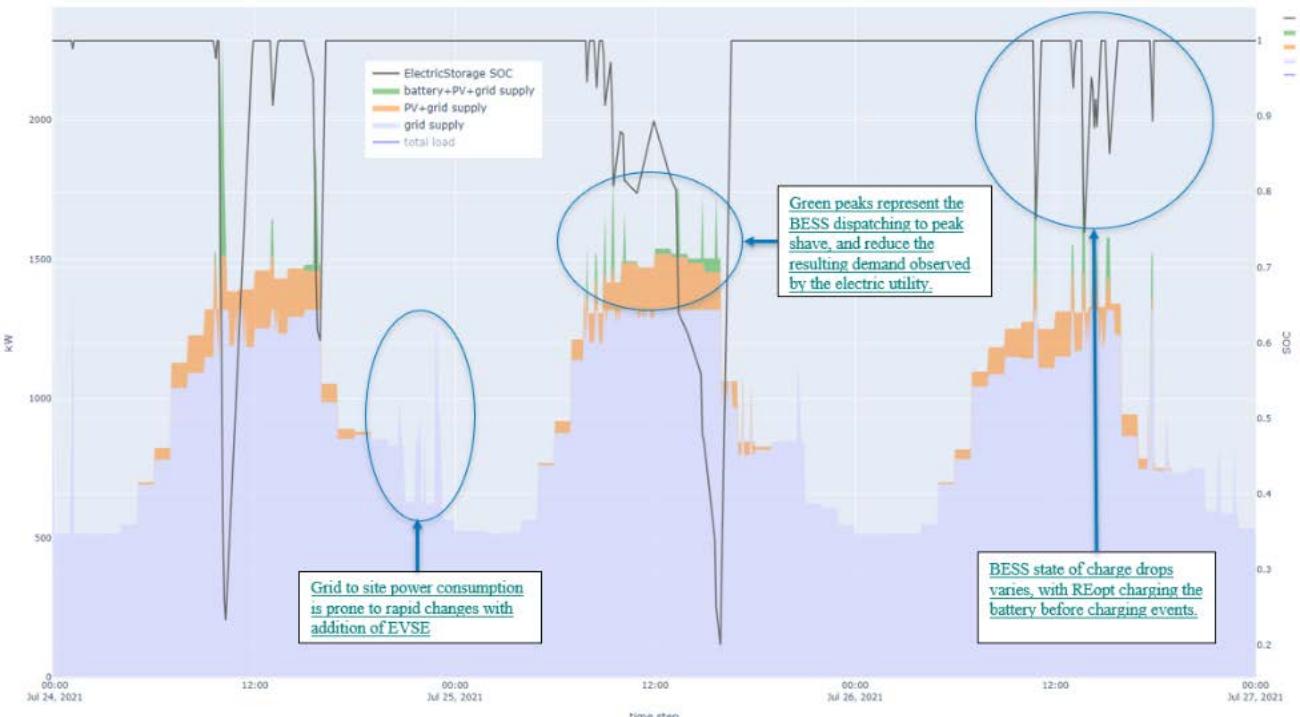
Figure 60. Example of solar PV and BESS dispatch to meet site loads at ACY under the restricted rooftop area scenario.
Figure 63, Figure 64, and Figure 65 present the changes in measured monthly peak demand for all three sites due to the addition of charging loads, as well as the addition of any REoptrecommended DERs. Observe that for all the sites, the BAU+CH scenario has higher monthly peak demand compared to other scenarios.

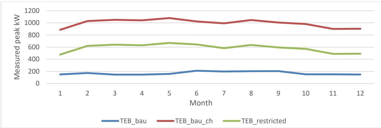
Figure 61. Monthly peak demand values at TEB for various scenarios.
As shown in Figure 63 for TEB, the monthly peak demand for the BAU+CH case increases 5 times compared to the case for BAU, while for cost-optimal restricted case, it decreases by 40% compared to the BAU+CH case.

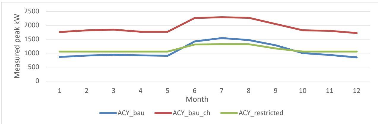
Figure 62. Monthly peak demand values at ACY for various scenarios.
As shown in Figure 64 for ACY, the monthly peak demand for the BAU+CH case increases around 2 times compared to the case for BAU, while for cost-optimal restricted case, it decreases back to being close to the BAU case.

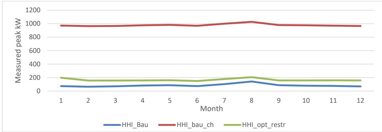
Figure 63. Monthly peak demand values at HHI for various scenarios.
As shown in Figure 65 for HHI, the monthly peak demand for the BAU+CH case increases approximately 10 times compared to the case for BAU, while for cost-optimal restricted case, it decreases by approximately 80% compared to the BAU+CH case.
Table 26, Table 27, Table 28, Table 29, and Table 30 present the detailed financial and electric tariff results for all three sites for both optimal and optimal restricted scenarios.
Table 26. Comparison of Financial Results for ACY’s BAU+CH and Optimal Scenarios
| Scenario | Utility Bill Component | t Tax? | Time Frame | Cost | % Difference |
| BAU+CH | Demand charges | After tax | Life cycle | $5,156,925 | NA |
| Optimal | Energy charges | After tax | Life cycle | $6,657,552 | NA |
| Demand charges | After tax | Life cycle | $1,812,223 | 64.86% |
| BAU+CH | Energy charges | After tax | Life cycle | $3,983,845 | 40.16% |
| Demand charges | Before tax | Year1 | $430,676 | NA |
| Energy charges | Before tax | Year 1 | $556,000 | NA |
| Optimal | Year 1 bill | Before tax | Year1 | $993,633 | NA |
| Demand charges | Before tax | Year 1 | $151,346 | 64.86% |
| Energy charges | Before tax | Year1 | $332,707 | 40.16% |
| Year 1 bill | Before tax | Year1 | $491,010 | 50.58% |
| BAU+CH | Life cycle cost | NA | NA | $11,897,768 | NA |
| Optimal | Life cycle cost | NA | NA | $9,006,628 | 24.30% |
As presented in Table 26, in ACY’s utility bill cost estimation, demand charges are a major contributor to overall cost, which reduces significantly between the optimal scenario and the BAU+CH scenario. Note that the Year 1 bill reduces by approximately half with the optimal scenario compared to the BAU+CH scenario. The life cycle cost reduces for the cost-optimal scenarios by 24% compared to the BAU+CH scenario, resulting in an NPV of approximately \$2.89 million.
Table 27. Comparison of Financial Results for ACY’s BAU+CH and Restricted Optimal Scenarios
| Scenario | Utility Bill Component | Tax? | Time Frame | Cost | % Difference |
| BAU+CH | Demand charges | After tax | Life cycle | $5,156,925 | NA |
| BAU+CH | Energy charges | After tax | Life cycle | $6,657,552 | NA |
| Optimal_restricted | Demand charges | After tax | Life cycle | $2,976,809 | 42.28% |
| Optimal_restricted | Energy charges | After tax | Life cycle | $6,218,360 | 6.60% |
| BAU+CH | Demand charges | Before tax | Year1 | $430,676 | NA |
| BAU+CH | Energy charges | Before tax | Year1 | $556,000 | NA |
| BAU+CH | Year 1 bill | Before tax | Year 1 | $993,633 | NA |
| Optimal_restricted | Demand charges | Before tax | Year1 | $248,605 | 42.28% |
| Optimal_restricted | Energy charges | Before tax | Year 1 | $519,321 | 6.60% |
| Optimal_restricted | Year 1 bill | Before tax | Year 1 | $774,883 | 22.02% |
| BAU+CH | Life cycle cost | NA | NA | $11,897,768 | NA |
| Optimal_restricted | Life cycle cost | NA | NA | $10,142,110 | 14.76% |
Per Table 27, restricting rooftop area at ACY results in reduced utility bill cost savings. Energy charge savings drop from 40% to 6% because of reduction in PV system size. This reduced PV size also results in a considerably smaller battery capacity, as the battery has to purchase more energy from the grid for charging, which is expensive. Therefore, although demand charge reduction is diminished (drops from 64% to 42%), it is still a major cost-saving avenue at ACY.
Table 28. Comparison of Financial Results for TEB’s BAU+CH and Optimal Scenarios
| Scenario Utility Bill Component | Tax? | Time Frame | Cost | % Decrease |
| BAU+CH | Demand charges | After tax | Life cycle | $511,685 | NA |
| BAU+CH | Energy charges | After tax | Life cycle | $2,303,581NA | |
| BAU+CH | Summer demand charges After tax | | Life cycle | $414,742 | NA |
| Optimal | Demand charges | After tax | Life cycle | $71,585 | 86.01% |
| Optimal | Energy charges | After tax | Life cycle | $814,864 | 64.63% |
| Optimal | Summer demand charges After tax | | Life cycle | $59,247 | 85.71% |
| BAU+CH | Demand charges | Before tax | Year 1 | $42,733 | NA |
| BAU+CH Energy charges | Before tax Year 1 | | $192,381 | NA |
| BAU+CH | Summer demand charges | Before tax Year 1 | | $34,636 | NA |
| BAU+CH Year 1 bill | | Before tax Year 1 | | $269,751 | NA |
| Optimal | Demand charges | Before tax Year 1 | | $5,978 | 86.01% |
| Optimal | Energy charges | Before tax Year 1 | | $68,053 | 64.63% |
| Optimal | Summer demand charges E | Before tax Year 1 | | $4,948 | 85.71% |
| Optimal | Year 1 bill | Before tax Year 1 | | $78,979 | 70.72% |
| BAU+CH Life cycle cost | | NA | NA | $3,369,220 | NA |
| Optimal | Life cycle cost | NA | NA | $2,44,09027.46% | |
Per Table 28, REopt-recommended system sizes under the optimal scenario can provide up to 70% cost savings in the Year 1 electric utility bill for TEB. Similar to ACY, these savings include demand charge reductions (both summer and annual demand charges) and energy charge reductions.
Table 29. Comparison of Financial Results for TEB’s BAU+CH and Restricted Optimal Scenarios
| Scenario | Utility Bill Component | Tax? | Time Frame | Cost | % Decrease |
| BAU+CH | Demand charges | After tax | Life cycle | $511,685 | NA |
| BAU+CH | Energy charges | After tax | Life cycle | $2,303,581 | NA |
| BAU+CH | Summer demand charges | After tax | Life cycle | $414,742 | NA |
| Optimal_restricted Demand charges | | After tax | Life cycle | $302,068 | 40.97% |
| Optimal_restricted | Energy charges | After tax | Life cycle | $2,304,818 | -0.05% |
| Optimal_restricted | Summer demand charges | After tax | Life cycle | $250,584 | 39.58% |
| BAU+CH | Demand charges | Before tax Year 1 | | $42,733 | NA |
| BAU+CH | Energy charges | Before tax Year 1 | | $192,381 | NA |
| BAU+CH | Summer demand charges | Before tax Year 1 | | $34,636 | NA |
| BAU+CH | Year 1 bill | Before tax | Year 1 | $269,751 | NA |
| Optimal_restricted | Demand charges | Before tax | Year 1 | $25,227 | 40.97% |
| Optimal_restricted Energy charges | | Before tax Year 1 | | $192,485 | -0.05% |
| Optimal_restricted Summer demand charges | Before tax Year 1 | | $20,927 | 39.58% |
| Optimal_restricted Year 1 bill | | Before tax Year 1 | | $238,639 | 11.53% |
| BAU+CH | Life cycle cost | NA | NA | $3,369,220 | NA |
| Optimal_restricted Life cycle cost | | NA | NA | $3,260,2373.23% | |
When maximum PV system size is restricted for TEB to existing PV, per Table 29, the site now consumes more grid electricity than the BAU+CH scenario to perform energy arbitrage and peak demand reduction using the recommended battery. Absence of a site’s true load profile results in the site’s load being modeled as “net” load, where all existing PV capacity is already serving the true site load. Therefore, REopt is unable to allocate cheap PV energy for battery system charging, which results in a smaller recommended battery energy capacity for this scenario.
Table 30. Comparison of Financial Results for HHI's BAU+CH and Optimal Scenarios
| Scenario | Utility Bill Component | Tax? | Time Frame | Cost | % Decrease |
| BAU+CH | Demand charges | After tax | Life cycle | $503,403 | NA |
| BAU+CH | Energy charges | After tax | Life cycle | $422,376 | NA |
| BAU+CH | Other demand charges a | After tax | Life cycle | $679,284 | NA |
| Optimal | Demand charges | After tax | Life cycle | $85,461 | 83.02% |
| Optimal | Energy charges | After tax | Life cycle | $392,980 | 6.96% |
| Optimal | Other demand charges a | After tax | Life cycle | $101,376 | 85.08% |
| BAU+CH | Demand charges | Before tax | Year1 | $42,041 | NA |
| BAU+CH | Energy charges | Before tax Year 1 | | $35,274 | NA |
| BAU+CH | Summer demand charges | Before tax | Year 1 | $17,584 | NA |
| BAU+CH | System peak charges | Before tax Year 1 | | $146,373 | NA |
| BAU+CH | Year 1 bill | Before tax | Year1 | $245,446 | NA |
| Optimal | Demand charges | Before tax | Year 1 | $7,137 | 83.02% |
| Optimal | Energy charges | Before tax | Year1 | $32,819 | 6.96% |
| Optimal | Summer demand charges Before tax Year 1 | | | $3,510 | 80.04% |
| Optimal | System peak charges | Before tax | Year 1 | $16,528 | 88.71% |
| Optimal | Year 1 bill | Before tax | Year 1 | $64,168 | 73.86% |
| BAU+CH | Life cycle cost | NA | NA | $1,655,032 | NA |
| Optimal | Life cycle cost | NA | NA | $1,240,922 | 25.02% |
a Other demand charges include summer demand charges and transmission- and capacity-related demand charges over the analysis period of 25 years.
Per Table 30, the leading factor for utility bill savings at HHI is demand charge reduction performed by the battery. Given the site is charged for annual demand, summer demand, and its contribution to systemwide peak demand, the battery has a critical role at HHI in performing peak energy shaving. PV is not cost-effective at this site because the site operational load is very small in comparison to the peaky charging loads. The \~7% savings in energy charges are a result of battery performing energy arbitrage to charge when prices are low and discharge when prices are high due to the availability of variable per-time-step energy prices.
Table 31 presents the probability of surviving 4-hour outages for cost-optimal and cost-optimal restricted scenarios for all the sites. The survival probability drops considerably when area limitations are imposed (see ACY results). However, adding on-site resources such as the existing generator for HHI allows the optimal system to survive a 4-hour outage with near 100% likelihood. Resilience analysis is also discussed in Section 4: Discussion and Conclusions.
Table 31. Optimal Systems With High-Power, Short-Duration Batteries Do Not Provide Very High Probability of Surviving 4-Hour Outages
| Site | Scenario | Probability Of Surviving One 4-Hour Outage | Mean Critical Load | Resilience Benefit |
| ACY | Optimal | 65% | 333 kW | $866/outage |
| Optimal_restricted | 1.1% | $15/outage |
| TEB | Optimal | 41% | 194 kW | $318/outage |
| Optimal_restricted | 27% | $13/outage |
| HHI | Optimal | 71% | 38 kW | $108/outage |
| Optimal with generator | 99.6% | $151/outage |
Figure 66 shows the visualization of the probability of survival for different scenarios at different sites. Because HHI site has an on-site generator, it has the highest probability for the survival for longer outage duration. With the cost-optimal scenario for ACY and TEB, the probability of survival is less even for 1-hour-long outage due to higher load and limited on-site PV generation opportunity.

Figure 64. Visualizing the probability of survival for all optimal scenarios for all three sites.
## 3.5 Greenhouse Gas Emissions Impacts
GHG emissions resulting from electricity consumption at the ACY, TEB, and HHI sites are estimated using the methodology described in Section 2.4.
## 3.5.1 Summary of Results
Because all three sites included in this assessment are located in New Jersey, the emissions rates for grid electricity apply consistently to each site. In the attributional accounting approach, annual average emissions rates are used. These are meant to reflect the average emissions
intensity of the various power sources that supply New Jersey loads over a full year. NREL Cambium’s mid-case scenario projects that these annual average emissions rates will generally decrease between 2024 and 2050 (Figure 67). However, by 2050, the average megawatt-hours of electricity consumed in New Jersey is projected to cause over 100 kg CO2e to be emitted.
In the consequential accounting approach, marginal emissions rates are used to capture the emissions intensity of the power sources that operate to meet marginal changes in electricity demand. These emissions rates are generally much higher than annual averages because they reflect a small portion of time when only the least economical (i.e., “dirtiest”) power generation sources are operating. In other words, for every new kilowatt-hour of electricity consumption that does not match historical load profiles and has not been planned for by grid operators, the SRMER describes the emissions that would be caused by that change. Similarly, a reduction in electricity consumption (i.e., kilowatt-hours not consumed or a negative change) avoids emissions at the marginal rate. The NREL Cambium SRMERs for 2024–2050 are also shown in Figure 67 and indicate how much greater the emissions intensity is for marginal changes in electricity consumption.
As these projections forecast further into the future, LRMERs can be used to consider the structural changes to the power grid that would occur over time in response to a sustained change in load profile. Therefore, these values are generally less than the SRMERs, but still higher than the annual average emissions rates.

Figure 65. Grid electricity emissions rates for New Jersey, 2024–2050. Source: NREL 2022 Cambium, Mid-Case
With this being said, emissions rates are only half of the emissions equation. The volume of electricity consumed—particularly the amount sourced by the power grid—is the primary factor influencing GHG emissions. In the calculations for each site, attributional accounting methods use the REopt-modeled total electricity consumed from the grid in each scenario along with the annual average emissions rate to estimate the total GHG emissions footprint in each scenario.
To provide a different angle on that analysis, consequential accounting methods make comparisons between scenarios to estimate how the change in grid electricity consumption from one scenario to another would cause or avoid marginal emissions. These comparisons are done in two steps. First, BAU is compared with BAU+CH to indicate the marginal emissions that would be caused by increasing site electricity consumption with eVTOL charging loads. BAU+CH then becomes the “new” baseline for comparison against Optimal and Optimal\_Restricted, respectively. Optimal consists of REopt-modeled electricity consumption at the site with costoptimal solar PV and battery storage supplementing grid electricity to power the site loads (including eVTOL charging loads in BAU+CH). Optimal\_Restricted is identical to Optimal, except for reductions to the PV system size to account for restrictions to available area for the installation of the PV array at the site. In each of these comparisons, Optimal and Optimal\_Restricted assume that changes in grid-sourced electricity compared to BAU+CH generally indicate the avoidance of emissions at the marginal emissions rate (i.e., the marginal power plants were not forced to operate in response to this change in site electricity demand because the on-site solar PV and battery system supplied the load).
## 3.5.1.1 Atlantic City Airport
The attributional accounting of GHG emissions at ACY found that the cost-optimal PV+BESS solution (Optimal) would offset the additional grid electricity consumption needed for the eVTOL charging (and more), resulting in ACY’s emissions footprint from electricity consumption to reduce by approximately one-third compared to BAU+CH. However, when REopt modeling considered the site restrictions for solar PV (Optimal\_Restricted), it computed a smaller system size than the cost-optimal system size in Optimal. This results in a smaller anticipated reduction in GHG emissions, but still offsets the increase in emissions seen in BAU+CH. Figure 68 illustrates the projected GHG emissions footprint in each scenario from 2024 through 2050.

Figure 66. Attributional accounting of GHG emissions from electricity consumption at ACY.
From the perspective of consequential emissions accounting, a key metric to communicate is the avoided emissions when comparing Optimal and Optimal\_Restricted to BAU+CH. In Optimal and Optimal\_Restricted, ACY site electricity loads, including eVTOL charging loads, are supplied by a mix of grid electricity, on-site solar PV generation, and battery storage discharge (which is charged by either grid or PV power). In BAU+CH, all site loads, including eVTOL charging loads, are supplied by grid electricity. The avoided emissions in all these cases are associated with the grid electricity that would not be consumed in Optimal and Optimal\_Restricted. To illustrate this with an example, consider the assumption that the siterestricted PV+BESS is installed at ACY (Optimal\_Restricted). The consequential accounting of avoided emissions in Optimal\_Restricted compared to BAU+CH in 2024 would be:
## ???? ???? ???????????????????????????????????????????? ???? 2024 = 5,835,470 ????????ℎ
Where:
$$
\begin{array} { c } { { L o a d _ { g r i d } = 5 , 4 5 0 , 3 7 9 k W h \mid L o a d _ { P V } = 3 8 5 , 0 9 1 k W h } } \\ { { L o a d _ { g r i d } + L o a d _ { P V } = 5 , 8 3 5 , 4 7 0 k W h } } \end{array}
$$
Note that $L o a d _ { g r i d }$ represents the load supplied by the grid, while $L o a d _ { P V }$ is the load supplied by PV generation.
In BAU+CH, the entire 5,835,470-kWh load is supplied by grid electricity. Therefore, the 385,091 kWh supplied by PV in Optimal\_Restricted avoids the same volume of electricity that would otherwise be supplied by the grid.
Using the SRMER for 2024, the calculation for these avoided emissions is:
$$
3 8 5 , 0 9 1 k W h * 7 2 9 . 5 \frac { k g C O _ { 2 } e } { M W h } = 2 8 0 , 9 2 4 k g C O _ { 2 } e
$$
In other words, by supplying 385,091 kWh of load with on-site solar PV in Optimal\_Restricted, ACY would avoid 280,924 kg of CO2e emissions that would otherwise be caused by consuming this electricity from the grid in BAU+CH.
It is important to note that the calculation of avoided emissions is not the same as an emissions reduction, because the avoided emissions analysis consists of two scenarios both occurring in the same future time period (the example above considered 2024).
## 3.5.1.2 Teterboro Airport
The attributional accounting of GHG emissions at TEB found that the cost-optimal PV+BESS solution (Optimal) would offset the additional grid electricity consumption needed for the eVTOL charging (and more), resulting in TEB’s emissions footprint from electricity consumption to reduce by approximately two-thirds compared to BAU+CH. However, when REopt modeling considered the site restrictions for solar PV (Optimal\_Restricted), it determined that the existing 640-kW solar PV located on-site does not allow for any additional generating capacity to be installed. Optimal\_Restricted, then, only differs from BAU+CH in the small increase in grid electricity consumption to charge a BESS. Figure 69 illustrates the projected GHG emissions footprint in each scenario from 2024 through 2050.
Teterboro Airport Estimated GHG Emissions Footprint from Grid-Sourced Electricity Consumption (2021 - 2050, by Scenario)

Figure 67. Attributional accounting of GHG emissions from electricity consumption at TEB.
From the perspective of consequential emissions accounting, there are likely no avoided emissions to report for TEB. It is assumed that Optimal is not feasible given the site constraints, and Optimal\_Restricted would result in a marginal increase in emissions compared to BAU+CH. However, if Optimal could be achieved, there would be significant emissions avoided compared to BAU+CH. The cost-optimal PV+BESS system in Optimal is modeled to provide 1,125,336 kWh of electricity to the site, which would otherwise be sourced from the grid in BAU+CH. Using the short-run marginal emissions factor for 2024 (729.5 kg CO2e/MWh), this avoided use of grid electricity corresponds with 820,933 kg of CO2e emissions avoided.
## 3.5.1.3 HHI
The attributional accounting of GHG emissions at HHI found that Optimal would increase emissions compared to BAU+CH because REopt analysis found no cost-optimal PV+BESS solution for the site. The increase in emissions is due to a slight increase in grid electricity consumption in Optimal for stand-alone on-site energy storage. Figure 70 illustrates the projected GHG emissions footprint in each scenario from 2024 through 2050.
HHI Heliport Estimated GHG Emissions Footprint from Grid-Sourced Electricity Consumption (2021 - 2050, by Scenario)

Figure 68. Attributional accounting of GHG emissions from electricity consumption at HHI.
With regard to consequential emissions accounting, HHI is similar to TEB in that there are no avoided emissions to report. Optimal and Optimal\_Restricted for HHI are identical and result in increased grid electricity consumption compared to BAU+CH. This increase in both of these scenarios corresponds with 167,731 kg of marginal CO2e emissions that would be caused.
## 3.6 Hazard and Cybersecurity Analysis
Detailed hazard analysis5 and cybersecurity impact analysis6 are published in a separate report and included in the appendix.
## 3.7 Job and Economic Development Impacts
Due to uncertainty about the actual regional purchase coefficients (RPCs) of the equipment and services required in the project—i.e., the portion purchased from New Jersey businesses versus from other U.S. states or imported—different scenarios were considered with varying RPC assumptions (Table 32).
Table 32. Materials and Services Sourcing Scenarios
| Scenario | New Jersey Allocation | Rest of U.S. Allocation | Rest of the World Allocation |
| Average RPCs | Average RPC by sector from USEEIO data | Average RPC by sector from USEElO data | Average RPC by sector from USEEIO data |
| 100% national | Imports allocated using Imports allocated using average RPC ratios | average RPC ratios | 0% |
| 100% New Jersey | 100% | 0% | 0% |
| 100% rest of the United States | 0% (except local government) | 100% | 0% |
“Average RPCs” assumes the average sourcing (local, rest of the United States, or imported) ratios from the USEEIO model to split the direct demand between national and foreign sources. This is a conservative assumption commonly used when local percentage of purchases is unknown. The “100% New Jersey” scenario is the most optimistic for the state, while the “100% rest of the United States” is the least beneficial. For each site, the average RPC estimates were broken down by direct, indirect, and induced effects for both New Jersey and the rest of the United States, as well as the possible range of total impacts from all scenarios. All monetary values shown are in 2021 dollars unless indicated.
Total charging infrastructure investments are estimated to create \$3.4 million of additional gross regional product in New Jersey and sustain 22 full-time equivalent (FTE) jobs during installation, while also creating \$4.3 million of gross regional product (GRP) for the rest of the United States and sustaining 26 jobs (FTE). Total microgrid infrastructure is expected to also generate \$3.5 million of additional GRP in New Jersey and sustain 22 jobs (FTE) during construction, while adding \$4.9 million to the rest of the U.S. GDP and employing 29 FTE. Finally, grid infrastructure investments are estimated to create \$3.5 million of GRP and 23 jobs in the state and increase GDP in the rest of the United States by \$3.9 million while sustaining 23 FTE jobs. The breakdown per site and range are shown in Figures 71–74.


Figure 69. Total construction impacts by category, ACY.
Figure 71 shows the impacts of each infrastructure project at ACY, with breakdowns for direct, indirect, and induced effects (top figures), as well as the expected range of impacts (bottom figures). Charging infrastructure is estimated to generate \$1.9 million of additional GRP and 12 FTE across the economy, of which 44% of GRP and 46% of jobs stay in New Jersey. The microgrid construction is expected to create \$3.1 million of additional GRP and 19 FTE (42% of GRP and 43% of jobs in New Jersey), while the grid expansion \$0.5 million of GRP and 3 FTE (47% of GRP and 49% of jobs in New Jersey). The full range of impacts is shown in the bottom two figures and depends on the actual suppliers’ locations (in-state or out-of-state).


Figure 70. Total construction impacts by category, TEB.
Figure 72 shows the impacts of each infrastructure project at TEB. Similar to ACY, charging infrastructure is estimated to generate \$1.9 million and 12 FTE across the economy, of which 44% of GRP and 46% of jobs stay in New Jersey. The microgrid construction is expected to create \$3 million of additional GRP and 19 FTE (42% of GRP and 43% of jobs in New Jersey), while the grid expansion \$0.1 million of GRP and 1 FTE (45% of GRP and 47% of jobs in New Jersey). The full range of impacts is shown in the bottom two figures and depends on the actual suppliers’ locations (in-state or out-of-state).


Figure 71. Total construction impacts by category, HHI heliport.
Figure 73 shows the impacts of each infrastructure project in the HHI heliport. Charging infrastructure is estimated to generate \$1.9 million and 12 FTE across the economy, of which 44% of GRP and 46% of jobs stay in New Jersey. The microgrid construction is expected to create \$2.2 million of additional GRP and 13 FTE (42% of GRP and 44% of jobs in New Jersey), while the grid expansion \$0.3 million of GRP and 2 FTE (47% of GRP and 49% of jobs in New Jersey). The full range of impacts is shown in the bottom two figures and depends on the actual suppliers’ locations (in-state or out-of-state).


Figure 72. Total construction impacts by category, HRHC.
Figure 74 shows the impacts of each infrastructure project at HRHC. Similar to the other sites, charging infrastructure is estimated to generate \$1.9 million and 12 FTE across the economy, of which 44% of GRP and 46% of jobs stay in New Jersey. There is no microgrid construction on this site, but grid expansion impacts (Feeder B) amount to \$6.6 million of GRP and 41 FTE (48% of the GRP impacts and 50% of jobs staying in New Jersey). The full range of impacts is shown in the bottom two figures and depends on the actual suppliers’ locations (in-state or outof-state).
Industries that benefit the most across direct and indirect supply chains are construction and electrical equipment manufacturing sectors in New Jersey (using average RPCs), and electrical equipment manufacturing and professional/technical services in the rest of the United States. Total earnings (direct, indirect, and induced) are concentrated in the construction and manufacturing industries in New Jersey and in manufacturing, technical services, finance, insurance, and real estate in the rest of the United States (Figure 75).

Figure 73. Total earnings by category, sector, and region.
Total charging infrastructure maintenance is expected to create \$36,700/year of additional GRP in New Jersey and sustain 0.5 FTE/year, while also creating \$64,500/year of GRP for the rest of the United States and sustaining 0.4 FTE/year. Total microgrid infrastructure is expected to generate \$8,800/year of additional GRP in New Jersey, sustaining 0.1 FTE/year, while adding \$23,500/year to the rest of the U.S. GRP and employing 0.1 FTE/year. Finally, grid infrastructure investments are estimated to create \$15,900/year of GRP and 0.2 FTE jobs/year in the state and increase GRP in the rest of the United States \$28,400/year while sustaining 0.2 FTE jobs/year. The breakdown per site and range of impacts are shown in Figures 76–79.


Figure 74. Total O&M impacts per year by category, ACY.
Figure 76 shows the annual impacts of maintaining the new infrastructure at ACY, with breakdowns for direct, indirect, and induced effects (top figures), as well as the expected range of impacts (bottom figures). Using average material sourcing shares (RPCs), charging infrastructure is estimated to generate \$25,000/yr of additional GRP and sustain 0.22 jobs (FTE) across the economy, of which 36% of GRP and 54% of jobs stay in New Jersey. The microgrid O&M is expected to create \$12,000/yr of additional GRP and 0.1 FTE (27% of GRP and 45% of jobs staying in New Jersey), while the grid expansion \$2,000/yr of GRP and 0.02 FTE (32% of GRP and 52% of jobs in New Jersey). The full range of impacts is shown in the bottom two figures and depends on the actual suppliers’ locations (in-state or out-of-state).


Figure 75. Total O&M impacts per year by category, TEB.
Figure 77 shows the annual impacts of maintaining the new infrastructure at TEB. Similar to ACY, using average material sourcing shares (RPCs), charging infrastructure is estimated to generate \$25,000/yr of additional GRP and sustain 0.22 jobs (FTE) across the economy, of which 36% of GRP and 54% of jobs stay in New Jersey. The microgrid O&M is expected to create \$12,000/yr of additional GRP and 0.1 FTE (27% of GRP and 45% of jobs staying in New Jersey), while the grid expansion \$400/yr of GRP and 0.01 FTE (28% of GRP and 46% of jobs in New Jersey). The full range of impacts is shown in the bottom two figures and depends on the actual suppliers’ locations (in-state or out-of-state).


Figure 76. Total O&M impacts per year by category, HHI heliport.
Figure 78 shows the annual impacts of maintaining the new infrastructure at the HHI heliport. Using average material sourcing shares (RPCs), charging infrastructure is estimated to generate \$25,000/yr of additional GRP and sustain 0.22 jobs (FTE) across the economy, of which 36% of GRP and 54% of jobs stay in New Jersey. The microgrid O&M is expected to create \$8,000/yr of additional GRP and 0.1 FTE (27% of GRP and 45% of jobs staying in New Jersey), while the grid expansion \$1,500/yr of GRP and 0.01 FTE (30% of GRP and 50% of jobs in New Jersey). The full range of impacts is shown in the bottom two figures and depends on the actual suppliers’ locations (in-state or out-of-state).


Figure 77. Total O&M impacts per year by category, HRHC.
Figure 79 shows the annual impacts of maintaining the new infrastructure at HRHC. Using average material sourcing shares (RPCs), charging infrastructure is estimated to generate \$25,000/yr of additional GRP and sustain 0.22 jobs (FTE) across the economy, of which 36% of GRP and 54% of jobs stay in New Jersey. There is no microgrid investment in this site, but the grid expansion is expected to add \$40,000/yr of GRP and 0.4 FTE (36% of GRP and 58% of jobs in New Jersey). The full range of impacts is shown in the bottom two figures and depends on the actual suppliers’ locations (in-state or out-of-state).
Industries that benefit the most annually from O&M are construction and electrical equipment manufacturing (for repairs) and finance, insurance, real estate, and health services (due to wage spending) in both New Jersey and the rest of the United States. Total earnings are concentrated in construction, manufacturing, health care (from induced effects), and government industries in New Jersey and in manufacturing, technical services, finance, insurance, and real estate in the rest of the United States (Figure 80).

Figure 78. Total annual earnings by category, sector, and region.
Figure 81 and Figure 82 show the average expected impact per category of infrastructure investment and O&M by dividing the total impacts by the number of sites in this study (top figures). The range of impacts (bottom figures) depends on the actual suppliers’ locations (instate or out-of-state). On average, we expect construction to create an additional \$0.1–\$1.2 million of GRP and 1–10 jobs (FTE) in New Jersey, and between \$0.8 and \$2.1 million of GRP and 4–18 jobs (FTE) in the rest of the United States, depending on suppliers’ locations (Figure 81).


CI: Charging Infrastructure M1: Microgrid Infrastructure GI: Grid Infrastructure


Figure 79. Total construction impacts by category, average.
Average impacts for maintenance vary significantly across project categories (Figure 82). Charging infrastructure creates the highest effects, \$1,000–\$14,000/yr of GRP employing 0.01– 0.16 FTE in New Jersey and \$11,000–\$25,000/yr of GRP employing 0.06–0.22 FTE in the rest of the United States. The lowest O&M average impact is from the microgrid infrastructure, creating \$100–\$6,000/yr of GRP employing up to 0.06 FTE per project in New Jersey and \$5,000–\$11,000/yr of GRP and 0.03–0.09 FTE in the rest of the United States.


Cl: Charging Infrastructure MI: Microgrid Infrastructure GI: Grid Infrastructure


Figure 80. Total O&M impacts per year by category, average.
## 4 Discussion and Conclusion
For this study, key aircraft operational, performance, and cybersecurity data were collected to model electrical charging demand. In terms of aircraft information, all the aircraft fit roughly within a 50 × 50-ft footprint. DC peak charging power ranges from 300 kW to 1 MW, and surveyed aircraft require 5% or more of onboard energy capacity for takeoffs. Vertiport locations were chosen considering viable use cases. These locations include general aviation (commercial service and reliever), large heliport, parking garage, and hospital. From these sites, existing electrical infrastructure, resiliency, cybersecurity, electrical load, and utility metered and bill data were requested; among these, only utility bills were received and used to estimate current electrical load and utility tariff information. Considering the received information, vertiports should plan for 1-MW (and potentially higher) chargers to align market speed of deployment with utility upgrade timelines.
An agent-based model was developed to determine charging demand and flight schedule considering the operational philosophy of transportation network companies (i.e., Uber and Lyft), which is based on passenger demand and passenger-centric. Note that this is only one approach; other methods can be considered following fixed routes and flight schedules. The model was used to simulate the operation of a system of seven vertiports serving around 1,400 passengers with 34 eVTOL aircraft and approximately 1,170 flights per day. The passenger schedule was generated by applying weights to passenger party size, origin, routes, and time of request at the origin. The potential scenario for number of passengers was obtained by simulating varying passenger demand and optimal wait time for the passenger and airborne time, considering the aircraft fleet and charging infrastructure at the sites. Peak charging demand depends on the number of charging stations simulated for constrained and unconstrained charging scenarios, but energy used for charging did not differ between scenarios. The time for charging or peak charging demand depends on the weight assigned for passenger time of request at the origin. Charging was based on a first-come, first-served basis with the least required coordination, but peak charging demand can be optimized and passenger throughput can be increased with managed charging. For most sites, the addition of charging demand significantly increased overall electrical demand, thus requiring analysis of the impact on grid operation/infrastructure, utility bills, and GHG emissions.
To perform grid impact analysis, realistic test feeders were utilized to conduct a grid power flow simulation study in the absence of actual utility feeder models. The impact on grid operation parameters due to the addition of charging demand varies significantly across sites. Aircraft charging at ACY and TEB created substantial undervoltage and overloading of site transformers and lines. Charging at the HHI site created comparatively minor undervoltage, and HRHC had the least impact on voltage and transformer loading. However, the existing transformers and service lines at all sites are heavily overloaded. eVTOL charging at sites such as ACY would potentially lead to undervoltage at other parts of the feeders as well. In general, introducing aircraft charging loads will potentially create grid issues such as undervoltage and thermal overloading. Therefore, it is essential to conduct a grid impact study to determine the potential impacts and identify solutions for smooth integration of aircraft charging loads. In conclusion:
• eVTOL charging is likely to increase site load demand 6 to 7 times in most cases, but the infrastructure is usually designed to withstand a maximum of only 2–3 times the present demand. Therefore, eVTOL charging would significantly overload present systems. In some cases, such as the HRHC site, eVTOL charging is less than 15% of the present load, causing no major impact with the additional charging load.
Existing airport electrical infrastructure such as electrical lines and transformers may not have sufficient capacities to withstand aircraft charging loads. This is clear from the simulation study with sites like ACY, TEB, and HHI, where the transformers and lines are heavily overloaded.
Thermally limited electrical infrastructure, such as lines and transformers, would need to be upgraded to integrate eVTOL charging loads and maintain power quality. Recent supply chain issues and labor and raw material shortages have increased the lead time for transformer procurement from weeks to over 2 years (U.S. Department of Energy Office of Policy 2022). This will prove to be a challenge to perform the necessary upgrades and should be factored in the planning process.
Integrating aircraft charging demand on existing airport infrastructure will lead to severe undervoltage that could potentially cause equipment malfunction and power interruptions.
For some cases, line and transformer infrastructure upgrades can resolve undervoltage violations in the feeder; in other cases, traditional voltage mitigation options like OLTC, capacitor, and regulator setting exploration are needed to mitigate voltage violations. Note that where PV is included, certain inverter settings may improve high or low voltage (e.g., volt/VAR). Frequent and high-voltage fluctuations due to eVTOL charging could lead to repeated OLTC tap changes, causing hunting. A detailed analysis should therefore be conducted before installing, and careful inspection, testing, and maintenance of the installed OLTC is needed to ensure continued operation. The nature of the feeder and magnitude of overloads can also lead to cases where traditional voltage mitigation options are unable to resolve the extreme scenarios, and other voltage management solutions need to be explored.
Utilizing on-site energy storage and generation to support eVTOL charging can also be a potential solution to mitigate grid issues.
The addition of EVSE can also lead to considerable increases (+17% to +305%) in electric utility bills for sites. Furthermore, EVSE loads have the potential to push sites to alternate rate tariffs or change how peak demand is determined, which can also cause demand charges to spike.
Results from the REopt analyses show that short-duration, high-power batteries are cost-optimal when it comes to serving loads similar in nature to EVSE. Such types of BESS can discharge and perform peak shaving to reduce charging peaks and perform some energy arbitrage to provide cost savings during charging events and in other hours of the day. Based on results from the optimal restricted scenarios, the biggest impact of optimal, short-duration, high-power BESS occurs for demand charges where sites can save about 40% for both TEB and ACY and about 80% for HHI in comparison to BAU+CH scenarios. The value of DERs would grow if EVSE loads were being considered in a region served by utilities like Pacific Gas and Electric, which have both seasonal and time-of-day variation in their demand and energy charges.
The results for HHI consider PSE&G’s Basic Generation Service capacity and transmission charges and show that on-site DERs could help reduce consumption during systemwide peak demand events, thereby providing significant cost savings on top of monthly demand charge savings. Such charges are applicable to commercial sites across many states in a variety of forms. Pacific Gas and Electric’s peak day pricing, Electric Reliability Council of Texas’s 4CP charges, and PJM’s 5CP charges are additional examples of such cost recovery methods that can constitute a significant portion of the increase in a site’s electric bill if EVSE loads are added without on-site DERs.
Per Section 2.3.2, 4-hour outage durations provide a conservative estimate on the duration of outages expected at sites modeled in this report, which average approximately 2 hours per interruption. On-site DERs for cost-optimal scenarios do not provide a high probability of surviving 4-hour outages during the year while maintaining full operations. Adding dispatchable technologies such as generators can improve these probabilities, but generators add the uncertainty of fuel prices and on-site fuel burn pollution. Instead, higher-duration batteries can be considered to provide increased resiliency. Installing a larger battery reduces the NPV of a given system, but this drop due to additional capital expenses should be weighed against other financial factors such as outage resilience benefits and avoided cost of pollution from on-site fuel burn.
On-site DERs can provide cost savings and resilience to sites considering adding EVSE loads, but they cannot avoid rapid variations in grid-to-site power consumption. Therefore, utilities like PSE&G are likely to be more aggressive in determining peak demand per month and utilizing 5- minute time intervals.
Given that REopt has perfect foresight, if the on-site system controllers are unable to dispatch the DER in time for EVSE peaks, the site can see significant cost increases despite having on-site DERs. Additionally, failure of on-site controllers to dispatch DERs to cut back grid-to-site power consumption during systemwide peak events can result in a large cost to the site despite on-site DERs for multiple months during the year. Therefore, if a DER controller’s dispatch strategy is not aligned with eVTOL charge events and systemwide peak hours, a site could see considerable increases in demand charges. Alternatively, eVTOL charging could be aligned to maximize charging during overnight hours or when demand charges are currently at their lowest. Doing so could provide the margin for difference between how REopt dispatches DERs versus how on-site controllers might dispatch DERs under real-world conditions.
Due to a lack of detailed electricity rate information, monthly averaged energy costs were used to run REopt for the ACY and TEB sites. If these sites were actually seeing energy prices fluctuate with time of day, use of this “flat” monthly energy charge could negatively impact the costoptimal system sizing for BESS by reducing opportunities for energy arbitrage. Furthermore, optimal PV system sizing can be impacted if the flat energy prices are lower than what the site really gets billed. Sensitivity can be performed on system ownership models and technoeconomic assumptions to assess system cost optimality under various scenarios. This analysis can also be approached from a regional or multistate perspective instead of site-specific perspectives. For example, EVSE charging events at each of the three sites can be scheduled with consideration for the respective electric utility rates. Paying attention to systemwide peaks and levels of congestion across various nodes in the grid can allow EVSE charging events to be utilized to avoid potentially expensive charge events (or properly price them) and contribute to grid safety and reliability as a virtual power plant, thereby creating another value stream for the vertiports. Additionally, EVSE loads could be diverted to regions with surplus clean energy generation to benefit from cheap energy.
While there are many opportunities to reduce GHG emissions at the assessed sites, the specific focus within the context of this study pertains only to site electricity use. Consequently, there are two main pathways to reduce GHG emissions beyond the results reported here:
• Reductions in the overall consumption of electricity at each site:
o The assessment of GHG emissions for this analysis only considered increased site electricity consumption to serve eVTOL charging loads. However, a more holistic assessment would consider energy conservation and energy efficiency opportunities throughout each site. This would involve a review of building heating and cooling loads, lighting, process loads, etc. Any reductions in sitewide electricity consumption would result in reduced demand for grid electricity and associated GHG emissions.
• Reductions in the emissions intensity of the electricity consumed at each site:
o Any additional on-site renewable electricity generation in addition to the PV modeled for this analysis would offset the need for grid electricity, therefore reducing the overall emissions intensity of the sites’ electricity consumption profiles.
o Along with this, the grid itself may increase or decrease its emissions intensity over time with the retirement and construction of power generation stations. If the New Jersey power grid ends up having a lower emissions intensity than the emissions factors assumed in this analysis, the actual emissions caused by each site’s electricity consumption may be lower than projected.
Further analysis of GHG emissions could potentially yield additional opportunities for reductions by investigating the following:
• Holistic, sitewide energy planning and management through a comprehensive energy audit and GHG emissions inventory.
A similar analysis of site electricity use, eVTOL charging loads, and PV+BESS system optimization, but with a more granular temporal analysis.
This assessment considered annual values for the GHG emissions analysis, but monthly, daily, or hourly time scales uncover additional details about time of use, alignment of site loads with PV generation, and the hourly emissions intensity of the regional power grid. With respect to GHG emissions in particular, hourly emissions factors highlight variations in how “clean” or “dirty” the grid electricity is depending on the season and time of day. This analysis could help fine-tune the PV+BESS sizing and charging protocol, as well as the strategy for eVTOL charging protocol—both of which could yield further reductions in GHG emissions.
The construction and operation of new charging infrastructure for eVTOL aircraft in New Jersey is expected to create local jobs in multiple sectors, as well as stimulate both the local state economy and the rest of the United States. Depending on where materials and services are sourced, the combined impact of all charging infrastructure projects is estimated to generate up to \$4.6 million to New Jersey’s GDP and 29 jobs (FTE) during construction and up to an additional \$57,000 annually for maintenance, sustaining 0.6 FTE/yr. Microgrid investments can generate up to \$5 million to the local GDP and 31 jobs during construction, as well as \$18,000/yr of GDP and sustain 0.2 jobs/yr. Finally, grid expansion investments can add up to \$4.5 million to local GDP and 28 jobs during construction and \$25,000/yr of additional GDP and sustain 0.3 jobs/yr.
It is important to note that the presented estimates should be interpreted within the context of the assumptions employed in the modeling, as well as the limitations of the IO framework. The IO model employed for this analysis is static (representing economywide linkages and spending patterns in 2019) and does not account for dynamic impacts or changes over time. As such, the results presented here do not account for changes in the economic structure (including electricity grid) over time, meaning there are no economies of scale or technological changes in any industry. Moreover, the estimates are based on several assumptions about material sourcing. More accurate results can be obtained once suppliers and labor force hiring are determined for each project.
## References
Afshar, Shahab, Pablo Macedo, Farog Mohamed, and Vahid Disfani. 2021. “Mobile Charging Stations for Electric Vehicles — A Review.” Renewable and Sustainable Energy Reviews 152: 111654. https://doi.org/10.1016/j.rser.2021.111654.
Alternative Fuels Data Center. 2023. “Charging Infrastructure Procurement and Installation.” U.S. Department of Energy. Accessed Aug. 22, 2023. https://afdc.energy.gov/fuels/electricity\_infrastructure\_development.html.
American National Standards Institute (ANSI). 2011. “Electric Power Systems and Equipment - Voltage Ratings (60 Hertz).” ANSI C84.1-2011.
https://webstore.ansi.org/standards/nema/ansic842011.
Anderson, Kate, Dan Olis, Bill Becker, Linda Parkhill, Nick Laws, Xiangkun Li, Sakshi Mishra, et al. 2021. REopt Lite User Manual. Golden, CO: National Renewable Energy Laboratory. NREL/TP-7A40-79235. https://www.nrel.gov/docs/fy21osti/79235.pdf.
Antcliff, Kevin, Nicholas Borer, Sky Sartorius, Pasha Saleh, Robert Rose, Maxime Gariel, Joseph Oldham, et al. 2021. “Regional Air Mobility: Leveraging Our National Investments to Energize the American Travel Experience.” NASA white paper, 20210014033. https://ntrs.nasa.gov/citations/20210014033.
Argonne National Laboratory (ANL). 2021. “The U.S. Department of Energy Vehicle Technologies Office and National Aeronautics and Space Administration Joint Assessment of R&D Needs for Electric Aviation.” White paper.
https://anl.box.com/s/xr1wk53shzhvu4w3l57j90t1mhkq01b5.
BETA. 2023. “Charging.” Accessed March 2023. https://www.beta.team/charge/.
Black & Veatch. 2019. Powered for Take Off: NIA-NASA Urban Air Mobility Electric Infrastructure Study. Walnut Creek, CA: Black & Veatch. https://webassets.bv.com/2019- 11/NASA\_eVTOL\_Electric\_Infrastructure\_Study.pdf.
Black & Veatch. 2019. In Depot Charging and Planning Study. Walnut Creek, CA: Black & Veatch. https://ww2.arb.ca.gov/sites/default/files/2020- 09/C\_Burns\_McDonnell\_Foothill%20Transit\_ROP\_ADA08182020.pdf
Borlaug, B., M. Muratori, M. Gilleran, D. Woody, W. Muston, T. Canada, A. Ingram, H. Gresham, and C. McQueen. 2021. “Heavy-duty truck electrification and the impacts of depot charging on electricity distribution systems.” Nature Energy 6: 673–682. https://doi.org/10.1038/s41560-021-00855-0.
California Public Utilities Commission. 2021. “Electric System Reliability.” Feb. 17, 2021. https://www.cpuc.ca.gov/-/media/cpuc-website/transparency/commissioner-committees/ emerging-trends/2021/2021-02-17-electric-system-reliability-presentation---final.pdf.
DeSanti, Fred, Frank DiCola, William Wasnak, Brandon Murdock, and Dionisio Roman III. 2018. Atlantic City Microgrid Feasibility Study. Trenton, NJ: New Jersey Board of Public Utilities. https://nj.gov/bpu/pdf/energy/Atlantic%20City%20Feasibility%20Study%20+%20 Attachments.pdf.
Doo, Johnny T., Marilena D. Pavel, Arnaud Didey, Craig Hange, Nathan P. Diller, Michael A. Tsairides, Michael Smith, Edward Bennet, Michael Bromfield, and Jessie Mooberry. 2021. “NASA Electric Vertical Takeoff and Landing (eVTOL) Aircraft Technology for Public Services – A White Paper.” NASA Document Number 20205000636. https://ntrs.nasa.gov/api/ citations/20205000636/downloads/2021-08-20-eVTOL-White-Paper-Final\_V48.pdf.
Electric Power Research Institute (EPRI). 2023. “OpenDSS.” Accessed March 2023.
https://www.epri.com/pages/sa/opendss.
Federal Aviation Administration (FAA). 2018. “Design and Installation Details for Airport Visual Aids.” AC 150/5340-30. https://www.faa.gov/documentLibrary/media/ Advisory\_Circular/150-5340-30J.pdf.
. 2022. “Engineering Brief No. 105, Vertiport Design.” Memorandum, Sept. 21, 2022. https://www.faa.gov/sites/faa.gov/files/eb-105-vertiports.pdf.
Frithiof, Mattias, Philip Jonat, and Gael Le Bris. 2022. “Electrification of Airports From Landside to Airside.” WSP, May 25, 2022. https://www.wsp.com/en-us/insights/electrificationof-airports-from-landside-to-airside.
Gagnon, Pieter, Brady Cowiestoll, and Marty Schwarz. 2023. Cambium 2022 Scenario Descriptions and Documentation. Golden, CO: National Renewable Energy Laboratory. NREL/TP-6A40-84916. https://www.nrel.gov/docs/fy23osti/84916.pdf.
Goodrich, Kenneth H., and Colin R. Theodore. 2021. “Description of the NASA Urban Air Mobility Maturity Level (UML) Scale.” AIAA SciTech Forum.
https://ntrs.nasa.gov/citations/20205010189.
Greenhouse Gas Protocol. 2005. The GHG Protocol for Project Accounting. Washington, D.C.: World Resources Institute; Geneva, Switzerland: World Business Council for Sustainable Development. https://ghgprotocol.org/sites/default/files/standards/ghg\_project\_accounting.pdf.
Greenhouse Gas Protocol. 2007. Guidelines for Quantifying GHG Reductions from Grid-Connected Electricity Projects. Washington, D.C.: World Resources Institute; Geneva, Switzerland: World Business Council for Sustainable Development. https://ghgprotocol.org/sites/default/files/standards\_supporting/Guidelines%20for%20Grid-Connected%20Electricity%20Projects.pdf.
Hill, D.P., D. DeCarne, M. Metcalfe, C. Griffin, S. Wiggins, C. Metts, B. Bastedo, M.D. Patterson, and N.L. Mendonca. 2020. UAM Vision Concept of Operations (ConOps) UAM Maturity Level (UML) 4, Version 1.0.” New York, NY: Deloitte Consulting. https://ntrs.nasa.gov/citations/20205011091.
Hodge, Cabell, Jesse Bennett, Julian Bentley, and Leidy Boyce. 2022. Considerations for Department of Defense Implementation of Zero-Emission Vehicles and Charging Infrastructure. Golden, CO: National Renewable Energy Laboratory. NREL/TP-5400-81925. https://www.nrel.gov/docs/fy22osti/81925.pdf.
Jayaraj Rane, Bharatkumar Solanki, Scott Cary, Prateek Joshi, and Subhankar Ganguly. 2023. Overview of Potential Hazards in Electric Aircraft Charging Infrastructure. Golden, CO: National Renewable Energy Laboratory. NREL/TP-5R00-83429. https://www.nrel.gov/docs/fy23osti/83429.pdf
Jeffers, M., Kenneth Kelly, Timothy Lipman, Andre Fernandes Tomon Avelino, Caley Johnson, Mengming Li, Matthew Post, and Yimin Zhang. 2022. Comprehensive Review of California’s Innovative Clean Transit Regulation: Phase I Summary Report. Golden, CO: National Renewable Energy Laboratory. NREL/TP-5400-83232. https://www.nrel.gov/docs/fy23osti/83232.pdf.
Johnston, Tore, Robin Riedel, and Shivika Sahdev. 2020. “To Take off, Flying Vehicles First Need Places to Land.” McKinsey & Company. Aug. 31, 2020. https://www.mckinsey.com/industries/automotive-and-assembly/our-insights/to-take-off-flyingvehicles-first-need-places-to-land.
Kloss, Benedikt, and Robin Riedel. 2021. “Up in the Air: How Do Consumers View Advanced Air Mobility?” McKinsey & Company, June 1, 2021. www.mckinsey.com/industries/aerospaceand-defense/our-insights/up-in-the-air-how-do-consumers-view-advanced-air-mobility.
Lahr, M., Erin Coughlin, and Frank Felder. 2010. Economic Impacts of Energy Infrastructure Investments. New Brunswick, NJ: Rutgers University.
Lilium. 2020. “Designing a scalable vertiport.” July 2, 2020. https://lilium.com/newsroomdetail/designing-a-scalable-vertiport
Markel, Anthony, and Anuj Sanghvi. 2022. Addressing Electric Aviation Infrastructure Cybersecurity Implementation. Golden, CO: National Renewable Energy Laboratory. NREL/TP-5R00-82856. https://doi.org/10.2172/1906953.
National Academies of Sciences, Engineering, and Medicine (NASEM). 2018. Battery Electric Buses State of the Practice. Washington, D.C.: The National Academies Press. https://doi.org/10.17226/25061.
National Renewable Energy Laboratory (NREL). 2019. “DISCO Documentation.” https://nrel.github.io/disco/.
—. 2021. “Annual Technology Baseline.” Accessed March 2023. https://atb.nrel.gov/.
. 2023a. “Distribution Grid Integration Unit Cost Database.” Accessed March 2023. https://www.nrel.gov/solar/market-research-analysis/distribution-grid-integration-unit-costdatabase.html.
. 2023b. “EVI-EnSite: Electric Vehicle Infrastructure – Energy Estimation and Site Optimization Tool.” Accessed Aug. 22, 2023. https://www.nrel.gov/transportation/eviensite.html.
. 2023c. “FASTSim: Future Automotive Systems Technology Simulator.” Accessed Aug. 22, 2023. https://www.nrel.gov/transportation/fastsim.html.
. 2023d. “JEDI Transmission Line Model.” Accessed Aug. 22, 2023. https://www.nrel.gov/analysis/jedi/transmission-line.html.
. 2023e. “REopt: Renewable Energy Integration & Optimization.” Accessed Aug. 22, 2023. https://reopt.nrel.gov/.
. 2023f. “SMART-DS: Synthetic Models for Advanced, Realistic Testing: Distribution Systems and Scenarios.” Accessed March 2023. https://www.nrel.gov/grid/smart-ds.html.
Navigant. 2020. Economic Development Benefits of the Proposed Astoria Replacement Project. Washington, D.C.: Navigant. https://www.nrg.com/assets/documents/legal/astoria/00\_misc/ economic-development-NRG-6-2020.pdf.
Palmintier, Bryan, Meghan Mooney, Kelsey Horowitz, Sherin Abraham, Tarek Elgindy, Kwami Sedzro, Ben Sigrin, Jane Lockshin, Brady Cowiestoll, and Paul Denholm. 2021. The Los Angeles 100% Renewable Energy Study (LA100): Chapter 7. Distribution System Analysis. Golden, CO: National Renewable Energy Laboratory. NREL/TP-6A20-85428. doi: 10.2172/1958737.
Port Authority of New York and New Jersey (PANYNJ). 2023. “Airport Information.” Accessed March 2023. https://www.panynj.gov/airports/en/teterboro/teterboro-operations.html.
Schwab, Amy, Anna Thomas, Jesse Bennett, Emma Robertson, and Scott Cary. 2021. Electrification of Aircraft: Challenges, Barriers, and Potential Impacts. Golden, CO: National Renewable Energy Laboratory. NREL/TP-6A20-80220. https://www.nrel.gov/docs/fy22osti/80220.pdf.
Schweiger, Karolin, and Lukas Preis. 2022. “Urban Air Mobility: Systematic Review of Scientific Publications and Regulations for Vertiport Design and Operations.” Drones 6 (7): 179. https://doi.org/10.3390/drones6070179.
Schweiger, Karolin, Franz Knabe, and Bernd Korn. 2022. “An Exemplary Definition of a Vertidrome’s Airside Concept of Operations.” Aerospace Science and Technology 125: 107144. https://doi.org/10.1016/j.ast.2021.107144.
Sedzro, K. S. A., M. Emmanuel, and S. A. Abraham. 2022. “Generating sequential PV deployment scenarios for high renewable distribution grid planning.” 2022 IEEE International Conference on Power Systems Technology (POWERCON), Kuala Lumpur, Malaysia. doi: 10.1109/POWERCON53406.2022.9929337.
Uber Elevate. 2016. “Fast-Forwarding to a Future of On-Demand Urban Air Transportation.” https://evtol.news/\_\_media/PDFs/UberElevateWhitePaperOct2016.pdf.
U.S. Bureau of Economic Analysis (BEA). 2018. “Use Tables / Before Redefinitions / Margin Details.” Data file. https://apps.bea.gov/industry/xls/underlying-estimates/ Margins\_Before\_Redefinitions\_2007\_2012\_DET.xlsx.
U.S. Congress. 2022. Inflation Reduction Act of 2022. H.R. 5376, 117th Cong., Public Law 117– 169. https://www.congress.gov/bill/117th-congress/house-bill/5376/text.
U.S. Department of Energy Federal Energy Management Program (FEMP). 2023. “Electric Vehicles Toolkit.” Accessed Aug. 22, 2023. https://www.energy.gov/femp/electric-vehiclestoolkit.
U.S. Department of Energy Office of Energy Efficiency and Renewable Energy (EERE). 2023.
“Commercial Reference Buildings.” Accessed March 2023.
https://www.energy.gov/eere/buildings/commercial-reference-buildings.
U.S. Department of Energy Office of Policy. 2022. “DOE Actions to Unlock Transformer and Grid Component Production.” Oct. 20, 2022. https://www.energy.gov/policy/articles/doeactions-unlock-transformer-and-grid-component-production.
U.S. Department of Transportation. 2023. “EV Infrastructure Project Planning Checklist.” Updated May 5, 2023. https://www.transportation.gov/rural/ev/toolkit/ev-infrastructureplanning/project-planning-checklist.
U.S. Energy Information Agency. 2022. “Annual Electric Power Industry Report, Form EIA-861 detailed data files.” Oct. 6, 2022. https://www.eia.gov/electricity/data/eia861/.
U.S. Environmental Protection Agency (EPA). 2023a. “stateior.” GitHub data file.
https://github.com/USEPA/stateior.
. 2023b. “U.S. Environmentally-Extended Input-Output (USEEIO) Models.” https://www.epa.gov/land-research/us-environmentally-extended-input-output-useeio-models
Vascik, Parker D. 2020. “Systems Analysis of Urban Air Mobility Operational Scaling.” Doctoral thesis, Massachusetts Institute of Technology.
https://dspace.mit.edu/handle/1721.1/128057. Volocopter. 2023. “Voloport.” Accessed March 2023.
https://www.volocopter.com/solutions/voloport/. Walkowicz, Kevin, Andrew Meintz, and John Farrell. 2020. R&D Insights for Extreme Fast Charging of Medium- and Heavy-Duty Vehicles: Insights from the NREL Commercial Vehicles and Extreme Fast Charging Research Needs Workshop, August 27–28, 2019. Golden, CO: National Renewable Energy Laboratory. NREL/TP-5400-75705.
https://doi.org/10.2172/1604308.
Wang, W., D. Thom, K. S. Sedzro, S. A. Abraham, Y. Yao, J. Gu, and S. Ghosh. 2022. “PV Hosting Capacity Estimation: Experiences with Scalable Framework.” 2022 IEEE 49th Photovoltaics Specialists Conference (PVSC), Philadelphia, PA. doi: 10.1109/PVSC48317.2022.9938653.
Williams, Abigail. 2022. “How Airports and FBOs Are Starting to Upgrade Their Electrical Infrastructure.” Business Airport International, April 5, 2022. https://www.businessairportinternational.com/features/how-airports-and-fbos-are-starting-toupgrade-their-electrical-infrastructure.html.
## Bibliography
Bodini, Nicola, Dino Zardi, and Julie K. Lundquist. 2017. “Three-Dimensional Structure of Wind Turbine Wakes as Measured by Scanning Lidar.” Atmospheric Measurement Techniques 10: 2881–2896. https://doi.org/10.5194/amt-10-2881-2017.
Northeast UAS Airspace Integration Research Alliance (NUAIR). 2020. National Aeronautics and Space Administration Advanced Air Mobility (AAM) Vertiport Automation Trade Study. https://ntrs.nasa.gov/api/citations/20210009757/downloads/20210009757\_MAJohnson\_Vertiport TradeStudy\_final.pdf.
Northeast UAS Airspace Integration Research Alliance (NUAIR). 2021. High-Density Automated Vertiport Concept of Operations. https://ntrs.nasa.gov/api/citations/20210016168/ downloads/20210016168\_MJohnson\_VertiportAtmtnConOpsRprt\_final\_corrected.pdf.
Zhu, Lei, Jacob Holden, Eric Wood, and Jeffrey Gender. 2017. “Green Routing Fuel Saving Opportunity Assessment: A Case Study Using Large-Scale Real-World Travel Data.” Presented at the 2017 IEEE Intelligent Vehicles Symposium (IV), Los Angeles, CA, June 11–14. https://doi.org/10.1109/IVS.2017.7995882.
## Further Reading
Markel, Anthony, and Anuj Sanghvi. 2022. Addressing Electric Aviation Infrastructure Cybersecurity Implementation. Golden, CO: National Renewable Energy Laboratory. NREL/TP-5R00-82856. https://www.nrel.gov/docs/fy23osti/82856.pdf.
Rane, Jayaraj, Bharatkumar Solanki, Scott Cary, Prateek Joshi, and Subhankar Ganguly. 2023. Overview of Potential Hazards in Electric Aircraft Charging Infrastructure. Golden, CO: National Renewable Energy Laboratory. NREL/TP-5R00-83429.
https://www.nrel.gov/docs/fy24osti/83429.pdf.