MinerU OCR: FAA eVTOL Downwash/Outwash Surveys 2024

DOT/FAA/TC-24/42

Federal Aviation Administration William J. Hughes Technical Center Aviation Research Division Atlantic City International Airport New Jersey 08405

Electric Vertical Takeoff and Landing (eVTOL) Downwash and Outwash Surveys

December 2024

Final Report

This document is available to the U.S. public through the National Technical Information Services (NTIS), Springfield, Virginia 22161.

This document is also available from the Federal Aviation Administration William J. Hughes Technical Center at actlibrary.tc.faa.gov.

U.S. Department of Transportation Federal Aviation Administration

NOTICE

This document is disseminated under the sponsorship of the U.S. Department of Transportation in the interest of information exchange. The United States Government assumes no liability for the contents or use thereof. The United States Government does not endorse products or manufacturers. Trade or manufacturer's names appear herein solely because they are considered essential to the objective of this report. The findings and conclusions in this report are those of the author(s) and do not necessarily represent the views of the funding agency. This document does not constitute FAA policy. Consult the FAA sponsoring organization listed on the Technical Documentation page as to its use.

This report is available at the Federal Aviation Administration William J. Hughes Technical Center’s Full-Text Technical Reports page: actlibrary.tc.faa.gov in Adobe Acrobat portable document format (PDF).

1. Report No.DOT/FAA/TC-24/42	2. Government Accession No.	3. Recipient's Catalog No.
4. Title and SubtitleElectric Vertical Takeoff and Landing (eVTOL) DOWNWASH AND OUTWASHSURVEYS		5. Report DateDecember 2024
		6. Performing Organization Code
7. Author(s)Maria J. Muia, PhD*, Joshua Stanley*, Todd Anderson*, David Hall*, ZacharyShuman*, Jan Goericke**, Jagdeep Batther**, Zoren Habana**, Chengjin He**,and Hossein Saberi**		8. Performing Organization Report No.
9. Performing Organization Name and Address* Woolpert, Inc. **Advanced Rotorcraft Technology, Inc. (ART)4454 Idea Center Boulevard 6757 Fremont BlvdDayton, OH 45430 Fremont, CA 94538		10. Work Unit No. (TRAIS)
		11. Contract or Grant No.
12. Sponsoring Agency Name and AddressDepartment of TransportationFederal Aviation AdministrationOffice of Airports Safety and Standards800 Independence Avenue, S.W.Washington, DC 20591		13. Type of Report and Period CoveredFinal Report
		14. Sponsoring Agency CodeAAS-100
15. Supplementary NotesThe Federal Aviation Administration Aviation Research Division CORs were Ryan King and Russ Gorman.
16. AbstractAs part of the Federal Aviation Administration's (FAA) efort to establish vertiport design guidance for facilities intended toaccept powere i and special las rotorcra t is of gring iportance todeterine the risk factors rlated tovertical tkoffand landing (VTOL) operations and how to mitigate them.The airlow generated from the aircraft's rotors/propellers duringtakeoff and landing, nown as downwash and outwash (DWW), can pose sigificant risks to people and propert in the vicinityof aircraft operations. Downwash is the vertical, downward fow of air produced by rotors/propellrs while outwash is the lateralradial, outward airflow that occurs as the downwash contacts the landing surface. The negative impacts of DWOW may beexacerbated at vertiport locations in urban areas where high-volume, high-tempo operations are proposed because of the densepopulations and higher throughput in those areas. However, current research on the effects and mitigation of DW is limited.This report describes the collection and analysis of VTOL DWOW data and the need to mitigate associated risks.The most reliable way to obtain eVTOL DWOW data is from ful-scale aircraft surveys. This research measured the DWOW ofthree prototype eVTOL airraft for their maximum velocity at various locations on a vertiport. A ground-level aray and a verticalarray of ultrasonic three-dimensional anemometers were used for colleting the DWOW wind velocities. The DWOW surveyswere performed at various times and locations and conducted under daylight visual meteorlogical conditions. DWW wind datawere collected at each anemometer location on the ground or vertical sensor aray. The aircraft pilts performed several presetmaneuvers within the bounds of their respective aircraft fight envelopes.Analysis of the result included maximum instantaneusvelcities, moving means and moving standard deviations based on a 3-second ime frame, and a 3-second moving 95 percentile.The survey measurements for the three prototype eVTOL aircraf included in the research were compared to viscous vortexparticle method modeling and simulation where possible.
17. Key Words 18. Distribution StatementElectric vertical takeoff and landing, eVTOL, Advanced air This document is available to the U.S. public through themobility, AAM, Urban air mobility, UAM, Downwash and National Technical Information Service (NTIS), Springfield,outwash. Virginia 22161. This document is also available from theFederal Aviation Administration William J. Hughes TechnicalCenter at actlibrary.tc.faa.gov.
19. Security Classif. (of this report)Unclassified	20. Security Classif. (of this page)Unclassified	21. No. of Pages56	22.Price

ACKNOWLEDGEMENTS

The authors would like to thank Ryan King and William R. Gorman of the FAA Airport Technology Research and Development Branch for their insight and support. These activities would not have been possible without the willingness of the individual original equipment manufacturers to participate and make their aircraft available for this important aviation safety research. Special appreciation also goes to the individual flight test pilots, flight test support personnel, and the airport facility owners and operators where testing took place.

TABLE OF CONTENTS

Page
EXECUTIVE SUMMARY ix

1. INTRODUCTION 1
2. DESCRIPTION OF AIRCRAFT ANALYZED 5
3. INSTRUMENTS USED 5
   3.1 Horizontal Anemometer Array 6
   3.2 Vertical Array 7
   3.3 Ambient Anemometer 8
   3.4 Data Acquisition System 8
4. SCOPE OF TEST 8
5. METHODOLOGY 8
6. RESULTS 10
   6.1 eVTOL #1 10
   6.1.1 eVTOL #1 Horizontal Array Velocity Results 11
   6.1.2 eVTOL #1 Comparison to VVPM Modeling and Simulation 13
   6.2 eVTOL #2 15
   6.2.1 eVtOL #2 Horizontal Array Velocity Results 17
   6.2.2 eVTOL #2 Vertical Array Velocity Results 19
   6.2.3 eVTOL #2 Comparison to VVPM Modeling and Simulation 20
   6.3 eVTOL #3 34
   6.3.1 eVTOL #3 Horizontal Array Velocity Results 35
   6.3.2 eVTOL #3 Comparison to VVPM Modeling and Simulation 36
   6.4 eVTOL #4 38
7. CONCLUSIONS 40
   7.1 Modeling and Simulation 40
   7.2 DWOW Velocities 41
8. REFERENCES 44

LIST OF FIGURES

Figure Page
1 Example Wind Velocity and Blade Frequency Modeled 6
2 Ground Sensor Mounting 7
3 Vertical Array Mobile Cart 7
4 eVTOL #1 Maximum Velocity Recorded at Each Sensor Across All Surveys
in Plan View 12
5 eVTOL #1 Line Graph of Maximum Velocity Recorded at Each Sensor for
Each Survey 13
6 eVTOL #1 Modeled Total Velocity at 23 ft 14
7 eVTOL #1 Modeled Total Velocity at 46 ft 14
8 eVTOL #1 Modeled Total Velocity at 69 ft 15
9 eVTOL #2 Maximum Velocity Recorded at Each Sensor Across all Surveys
in Plan View 18
10 eVTOL #2 Line Graph of Maximum Velocity Recorded at Each Sensor
for Each Survey 19
11 Velocity Predictions at Sensor A2-S10 23
12 Velocity Predictions at Sensor A2-S20 23
13 Velocity Predictions at Sensor A2-S30 24
14 Velocity Predictions at Sensor B1-M40 24
15 Velocity Predictions at Sensor B1-M50 25
16 Velocity Predictions at Sensor C2-S10 25
17 Velocity Predictions at Sensor A2-S10 26
18 Velocity Predictions at Sensor A2-S20 27
19 Velocity Predictions at Sensor A2-S30 27
20 Velocity Predictions at Sensor B1-M40 28
21 Velocity Predictions at Sensor B1-M50 28
22 Velocity Predictions at Sensor C2-S10 29
23 Vertical Array Sensor Configuration 31
24 Tethered Test Case Correlation—Boxplots of Velocity Magnitude 32
25 Tethered Test Case Correlation—Time Histories of Velocity of Magnitudes 33
26 eVTOL #3 Maximum Velocity Recorded at Each Sensor Across All Surveys
in Plan View 35
27 eVTOL #3 Line Graph of Maximum Velocity Recorded at Each Sensor for
Each Survey 36
28 eVTOL #3 VVPM Resolution Sensitivity Study 37
29 Hybrid Method 38
30 Flow Field Sampling Points 39
31 Velocity Profile at 90° Radial 39
32 Maximum Velocity Measured by Sensor Distance to TLOF Center for All
eVTOL Aircraft Surveyed 42

LIST OF TABLES

1 Beaufort Wind Scale 1
2 Air Velocity Sensitivity Thresholds 3
3 Sensor Information from VVPM DWOW Simulation 5
4 Pilot Flight Tolerances 8
5 Data Summary Statistics Legend 9
6 eVTOL #1 Sensor Labels and Distances 10
7 eVTOL #1 Flight Details for Each Survey 10
8 eVTOL #1 Maximum Velocity Recorded at Each Sensor Across All Surveys 12
9 eVTOL #2 Sensor Labels and Distances 15
10 eVTOL #2 Flight Details for Each Survey 16
11 eVTOL #2 Maximum Velocity Recorded at Each Sensor Across All Surveys 19
12 eVTOL #2 Maximum Velocity Recorded for All Surveys 20
13 eVTOL #3 Sensor Labels and Distances 34
14 eVTOL #3 Flight Details for Each Survey 34
15 eVTOL #3 Maximum Velocity Recorded at Each Sensor Across All Surveys 36
16 Highest DWOW Velocity Measured 41
17 Overall Maximum Speeds Measured for All eVTOL Aircraft 43

AC Advisory Circular
AGL Above ground level
CFD Computer fluid dynamics
C.F.R. Code of Federal Regulations
DCA Downwash caution area
DWOW Downwash and outwash
EB Engineering Brief
eVTOL Electric vertical takeoff and landing
FAA Federal Aviation Administration
FATO Final approach and takeoff area
GPS Global Positioning System
GPU Graphic processing unit
MTOW Maximum takeoff weight
NASA National Aeronautics and Space Administration
NOAA National Oceanic and Atmospheric Administration
OEM Original equipment manufacturer
SA Safety area
TLOF Touchdown and liftoff area
VVPM Viscous vortex particle method
WMO World Meteorological Organization

EXECUTIVE SUMMARY

Electric vertical takeoff and landing (eVTOL) aircraft designs are emerging as a technology poised to increase mobility and simplify air travel. However, because the technology is new, research regarding the risks and dangers is limited. Very little data are available on the effects and potential risks of eVTOL aircraft including downwash and outwash (DWOW), which is the vertical airflow created by a rotor/propeller (downwash) and radial outflow of air once downwash meets the ground (outwash). eVTOL aircraft DWOW can pose significant risks to people and property and must be accounted for in vertiport design. The DWOW of an eVTOL aircraft varies by configuration. The most reliable way to obtain eVTOL DWOW data is from full-scale aircraft surveys. This research included surveys with eVTOL original equipment manufacturers (OEMs) to measure the velocity of their prototype aircraft’s DWOW in vertiport environments that complied with the touchdown and lift-off area (TLOF), final approach and takeoff area (FATO), and the safety area (SA) dimensions outlined in Federal Aviation Administration (FAA) Engineering Brief (EB) 105, Vertiport Design, for a square landing area.

This research employed a custom-made array of ultrasonic, three-dimensional anemometers surrounding the eVTOL vertiport test environment. The TLOF, FATO, and SA were based on the sizes outlined in FAA EB 105 for the controlling dimension of the aircraft being surveyed. GoPro® cameras were mounted outside the safety area to record the survey for reference should it be needed afterward. The DWOW surveys were conducted at various times and locations and performed under daylight, visual meteorological conditions. DWOW wind data were collected at each anemometer location on the ground or vertical sensor array. The eVTOL aircraft pilots performed several preset maneuvers based on input from the pilots and OEMs. Statistics were produced for maximum velocities (instantaneous) and moving means, moving standard deviations, and moving 95 percentiles based on a 3-second time frame. Ambient wind data were collected for reference, but no process was undertaken to subtract the ambient wind velocity from the wind generated by the DWOW.

The survey measurements for the eVTOL aircraft included in the research are compared to viscous vortex particle method (VVPM) modeling and simulation where possible. The current graphic processing unit (GPU) cards available limited the ability to model and simulate these aircraft because of the numerous propeller blades and their proximity to each other. Ultimately, 6 million particles were tracked for 30 revolutions. While particles closer to the aircraft are tracked effectively, their paths did not reach distances where DWOW velocities would be considered safe for people. These current limitations make VVPM alone an unlikely tool for forecasting where people and property will not be affected by high winds. A hybrid approach augmenting VVPM with global mass conservation may prove useful but has not been validated here.

The maximum velocities measured during the surveys taken varied from survey to survey and from aircraft to aircraft. The highest instantaneous maximum measured was almost 100 mph at 41 ft from the TLOF center. The highest moving 3-second 95th percentile was 84 mph at 23 ft from the TLOF center. Speeds of more than 60 mph were measured at 100 ft from the TLOF center.

The eVTOL aircraft surveyed produced high-velocity DWOW flow fields that could easily go beyond the safety area of a vertiport. The high-velocity DWOW of eVTOL aircraft should be considered when designing a vertiport because it can create safety risks to people, aircraft, equipment, and infrastructure, on and off the vertiport. eVTOL OEMs propose high-volume, high-tempo eVTOL operations in urban areas, which have an even greater potential of impacting bystanders with DWOW than traditional helicopters at heliports. In these target areas, the vertiports will likely be surrounded by dense populations in confined spaces and will experience higher throughput. Accordingly, it is recommended to mitigate DWOW by creating a downwash caution area (DCA). The DCA should be operational when and wherever DWOW velocities exceed 34.5 mph.

1. INTRODUCTION

Emerging electric vertical takeoff and landing (eVTOL) aircraft designs are abundant, complex, and vary in configuration based on their operational characteristics. These aircraft are positioned to be an industry gamechanger due to their potential for increased mobility. There are very little data on the performance of eVTOL aircraft including the effects of vertical airflow created by a rotor/propeller (downwash) and radial outflow of air once downwash meets the ground (outwash). Because DWOW can cause significant risks including property damage and personal injury, it is important that the Federal Aviation Administration (FAA) take into consideration the downwash and outwash (DWOW) of these aircraft when considering vertiport design guidance. Wind forces from DWOW are a risk to ground crew, passengers, aircraft, and adjacent people and structures (FAA, 2024).

Literature review identified several sources that address the dangers of the winds produced by DWOW. The National Weather Service uses the Beaufort Wind Scale to advise the public on the dangers of winds. Table 1 shows how the Beaufort Wind Scale estimates the strength of wind based on visual cues (National Oceanic and Atmospheric Administration [NOAA], 2023).

WMO = World Meteorological Organization
Table 1. Beaufort Wind Scale

Force	Wind(mph)	WMOClassification	Appearance of WindEffectsOn Water	Appearance of WindEffectsOn Land
0	<1	Calm	Sea surface smooth andmirror-like	Calm, smoke risesvertically
1	1-3	Light Air	Scaly ripples, no foamcrests	Smoke drift indicateswind direction, windvanes are still
2	4-7	Light Breeze	Small wavelets, crestsglassy, no breaking	Wind felt on face,leaves rustle, vanesbegin to move
3	8-12	Gentle Breeze	Large wavelets, crestsbegin to break, scatteredwhitecaps	Leaves and small twigsconstantly moving,light flags extended
4	13-18	ModerateBreeze	Small waves 1–4 ftbecoming longer,numerous whitecaps	Dust, leaves, and loosepaper lifted, small treebranches move
5	19-24	Fresh Breeze	Moderate waves 4–8 fttaking longer form, manywhitecaps, some spray	Small trees begin tosway
6	25-31	Strong Breeze	Larger waves 8–13 ft,whitecaps common, morespray	Larger tree branchesmoving, whistling inwires
7	32-38	Near Gale	Sea heaps up, waves 13–19ft, white foam streaks offbreakers	Whole trees moving,resistance felt walkingagainst wind
8	39-46	Gale	Moderately high (18–25 ft)waves of greater length,edges of crests begin tobreak into spindrift, foamblown in streaks	Twigs breaking offtrees, generallyimpedes progress
9	47-54	Strong Gale	High waves (23–32 ft), seabegins to roll, dense streaksof foam, spray may reducevisibility	Slight structuraldamage occurs, slateblows off roofs
10	55-63	Storm	Very high waves (29–41 ft)with overhanging crests,sea white with denselyblown foam, heavy rolling,lowered visibility	Seldom experienced onland, trees broken oruprooted, "considerablestructural damage"
11	64-73	Violent Storm	Exceptionally high (37–52ft) waves, foam patchescover sea, visibility morereduced
12	74+	Hurricane	Air filled with foam, wavesover 45 ft, sea completelywhite with driving spray,visibility greatly reduced

The FAA’s Rotorwash Analysis Handbook, Volume I – Development and Analysis (Ferguson, 1994), also discusses wind speed thresholds for danger. It indicates “that the majority of downwash and outwash related mishaps could be avoided if separation distances are maintained so that impacting DWOW-generated velocities do not exceed 30 to 40 knots (34.5 to 46.0 mph) across the ground” (Ferguson, 1994). The U.S. Army Research, Development, and Engineering Command Report, Rotorwash Operational Footprint Modeling (Preston et al., 2014), provides similar danger thresholds. Preston et al. (2014) indicate the caution zone for wind velocities for the general population is 33.6 to 44.7 mph while the hazard zone is 44.8 mph and greater, which is in line with the FAA Rotorwash Analysis Handbook. They conclude that rotorwash velocities above 40.3 mph can result in an airport/heliport incident. (Preston et al., 2014)

FAA Advisory Circular (AC) 150/5300-13B, Airport Design (2024), provides guidance for jet blast, which is the jet engine equivalence of DWOW. For airfield planning purposes, the FAA recommends applying the air velocities listed in Table 2, derived from the National Weather Service Beaufort Wind Scale (NOAA, 2023), as sensitivity thresholds at which safety risks increase (FAA, 2024). The items and areas of concern included in Table 2 represent the thresholds in which jet blast air velocities are of concern.

Table 2. Air Velocity Sensitivity Thresholds

Air Velocity Threshold	Items or Areas of concern
13–18 mph (21–29 km/h)	Unsecured trash, paper, and lightweight debris
24 mph (38 km/h)	Pedestrian areas (e.g., boarding passengers, General Aviationparking areas)
30 mph (48 km/h)	Light objects and empty containers, etc.Ramp personnel (e.g., marshals, baggage handlers)
35 mph (56 km/h)	General area aft of aircraft parking positionService roads and areas adjacent to parking positions and taxiroutes
50 mph (80 km/h)	Area behind aircraft after pushbackGeneral structures, passenger boarding equipment, etc.

Wind produced from aircraft propulsion units around vertiports can be turbulent and gusty and impact people and property. A sudden gust of wind can trigger a “startle response” where people react suddenly and perhaps put themselves in harm’s way. The FAA describes this as “an uncontrollable, automatic muscle reflex, raised heart rate, blood pressure, etc., elicited by exposure to a sudden, intense event that violates a pilot’s expectations” (FAA, 2017). It is associated with many aviation and other vehicle accidents. During a startle response, the brain skips all the normal sensory processing steps and “takes control of your body to protect you from danger” (Cleveland Clinic, 2023). This can cause a person to overreact to an event. “The ‘startle’ effect of being hit by a transient gust of wind can cause greater upset than being exposed to the same, constant wind velocity, and indeed that buffeting at certain frequencies can excite the human physiological response more easily than others” (Brown, 2023).

Low-to-the-ground, high-velocity winds can also pick up objects and project them through the air. This includes gravel, foreign object debris, and anything not secured to the ground. Such airborne debris can cause damage to aircraft and infrastructure in the vicinity. Dust, dirt, sand, and snow can also become airborne and recirculate through the propeller blades, causing brownout or whiteout environments (Ferguson, 1994). Brownouts and whiteouts can impede visibility and result in a loss of situational awareness.

Because of their potential to create safety risks to people, aircraft, equipment, and infrastructure, on and off the vertiport, the DWOW of eVTOL aircraft should be considered when designing a vertiport. The DWOW from the predecessor to eVTOL, the helicopter, has blown bystanders to the ground, resulting in injury and death (Werfelman, 2023; Australian Transport Safety Bureau, 2023; KABC Television, 2022). Helicopter DWOW has even injured people that the helicopter was sent to rescue (Swarts, 2016). Even when bystanders are aware of the potential for DWOW, they often do not understand the severity and risk associated with it (Werfelman, 2023).

An FAA aeronautical study will be required for most new vertiports as outlined in Title 14 Code of Federal Regulations (C.F.R.) Part 157, Notice of Construction, Alteration, Activation, and Deactivation of Airports. Part 157 states specifically what this study entails:

The FAA will consider matters such as the effects the proposed action would have on existing or contemplated traffic patterns of neighboring airports; the effects the proposed action would have on the existing airspace structure and projected programs of the FAA; and the effects that existing or proposed

manmade objects (on file with the FAA) and natural objects within the affected area would have on the airport proposal. While determinations consider the effects of the proposed action on the safe and efficient use of airspace by aircraft and the safety of persons and property on the ground, the determinations are only advisory. (Notice of Construction, Alteration, Activation, and Deactivation of Airports, 1991)

This study considers the safety of persons and property on the ground, and how DWOW can have a detrimental effect on them. OEMs propose high-volume, high-tempo operations in urban areas. Aircraft operating at vertiports in these areas have even greater potential for impacting bystanders with DWOW than helicopters because they will be surrounded by dense population in confined spaces and experience higher throughput (National Aeronautics and Space Administration [NASA], 2020; FAA, 2023b; Goodrich & Theodore, 2021). Accordingly, DWOW must be mitigated through either vertiport design features or operational procedures.

Vertiport design must consider the possibility of hazardous, high-velocity winds and identify safety measures to mitigate risks to people and property. However, the variances in designs and configuration types, and the complexity of emerging eVTOL aircraft make it difficult to develop a universal model for the prediction of the DWOW flow fields from these aircraft. Research has been conducted to understand rotor DWOW, but this understanding is mostly limited to one- and two-engine and rotary aircraft. The principles of DWOW wake turbulence and how the wake reacts with the surface, surrounding structures, and particularly with multiple other rotors or propellers, as is the case with eVTOL aircraft, is still not fully understood.

Computer modeling has been used extensively to predict the DWOW of single-rotor helicopters. eVTOL aircraft, however, differ significantly from helicopters and vary significantly in design and operational characteristics. Real-world data are limited for eVTOL aircraft compared to helicopters. The number of propellers on eVTOL aircraft and their varying locations make it very difficult to predict their DWOW flow fields, how they interact with each other, and how they interact with the aircraft fuselage. While computer fluid dynamics (CFD) methods, which involve analysis of aircraft performance, can provide impressive results, it can be difficult for use in eVTOL DWOW prediction because of the complexities inherent to eVTOL aircraft configurations with multiple propellers and complicated wake fields. Additionally, CFD methods are expensive and “suffer from gridinduced dissipation errors because of the numerical discretization over the flow field.” Even with advancements in CFD methods, “high computational costs and complicated equation setup still make these methods unfeasible for designers aiming for rapid feedback to optimize their models” (Lee et al., 2022).

Full-scale surveys are the most accurate way to determine the velocities of eVTOL DWOW flow fields on the vertiport environment. Accordingly, surveys were conducted with eVTOL OEMs to measure the velocity of each of their prototype aircraft’s DWOW in vertiport environments that complied with the TLOF, FATO, and the SA dimensions outlined in FAA (2023a) EB 105, Vertiport Design.

2. DESCRIPTION OF AIRCRAFT ANALYZED

This research included surveying three eVTOL aircraft, eVTOL #1, eVTOL #2, and eVTOL #3, for DWOW during 2023 and 2024. These aircraft varied in configuration, number of propulsion systems, blades per propulsion unit, and maximum takeoff weight (MTOW), all of which were less than 6,500 lb. They also varied in how they were controlled, by a pilot on board, remotely or computer programmed flight controls. The aircraft were all prototype, preproduction models.

3. INSTRUMENTS USED

This research employed three-dimensional, ultrasonic anemometers surrounding the eVTOL vertiport test environment. The TLOF, FATO, and SA were based on the sizes outlined in FAA EB 105 for the controlling dimension of the prototype aircraft being surveyed. GoPro cameras were mounted outside the safety area to record the survey for reference should it be needed afterward.

The selection of the sensors and their locations was predominantly based on preliminary VVPM simulation that was completed for two types of notional eVTOL aircraft. With the first principal formulation, VVPM solves for the vorticity field directly from the vorticityvelocity form of the incompressible Navier-Stokes equations using a Lagrangian approach. This is a natural way of solving vorticity-dominated flows because it only needs to be applied to regions with vorticity and does not require any grid generation effort. It also accurately resolves the vorticity in the flow field for long duration without artificial dissipation, as is often encountered by grid-based CFD solvers, while still capturing the wake distortion and physical diffusion due to air viscosity. It also takes a fraction of the computing time of CFD.

The VVPM and flow field simulations in hover mode and at different heights above the ground predicted wind velocities at various locations around the two notional aircraft. These predictions were to inform the following aspects of survey design:

• Predictions of flow velocities at the notional sensor locations to aid sensor type selection.

Estimate for the unsteadiness of local DWOW velocities at the notional sensor locations and frequency content of the flow for the determination of measurement sampling rate.

• Flow directionality at the sensor location for the definition of a required measurement range of the sensors to be used.

• Recommendation of vertical placement of sensor with the goal of capturing maximum outwash velocities.

Table 3 shows a summary of the sensor requirements determined from VVPM and flow field simulation.

Table 3. Sensor Information from VVPM DWOW Simulation

Sensor Property	Value
Sensor measurement range	0–95.5 mph
Sensor output rate	Approx. 40 Hz
Sensor angular measurement range	±30° horizontally and vertically
Horizontal placement	In zones with predicted high outwash
Vertical placement	Approx. 3 ft above the ground

The models provided quick insight into the predicted frequency, velocity magnitude, and the height above ground of the maximum DWOW velocities expected in the field. These models indicated that 100-Hz sensors were preferable closer to the aircraft and the lower cost 40-Hz sensors would be satisfactory farther away. The models also indicated that a 3-ft above ground level (AGL) sensor height for the ground array would generally cover the area of greatest wind velocities. Examples of the models’ output that lead to the selection of the anemometers are shown in Figure 1.

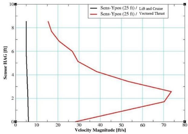
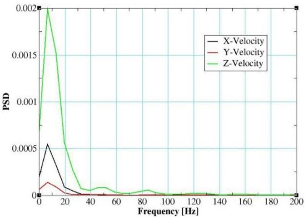
Figure 1. Example Wind Velocity and Blade Frequency Modeled

At the time this research was started, backlogs existed for many products that contained a computer chip, which limited the availability of anemometers, especially in the quantity sought for this project. LI-COR®’s Anemoment TriSonica® series was chosen based on its ability to meet all the technical requirements for the study and deliver the product in the desired time frame.

3.1 HORIZONTAL ANEMOMETER ARRAY

The horizontal sensor array consisted of a combination of LI-COR’s Anemoment TriSonica 100 Hz Sphere Wind Flux Sensors and TriSonica 40 Hz Mini Sensors. These sensors were located on two to four radials from the center of the TLOF at various distances.

The sensors were elevated to 3 ft above the grade and pipe mounted on a ½-inch DNS15 Schedule 10 pipe allowing for the wiring to run through the pipe, which was then mounted to a metal base via a frangible coupling. The bases included leveling mounts and added water weights (see Figure 2).

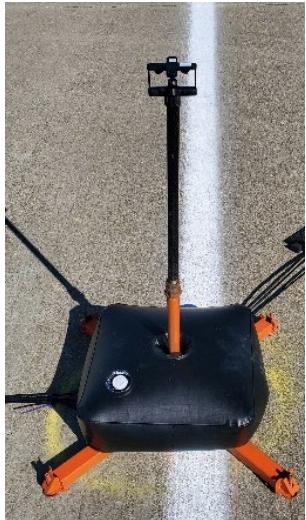
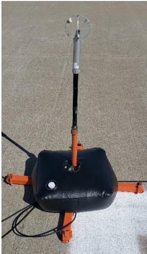
Figure 2. Ground Sensor Mounting

The TriSonica 100 Hz Spheres (right image in Figure 2) and 40 Hz Mini Sensors (left image in Figure 2) measured and recorded wind speed and direction in three dimensions of airflow. The 40 Hz Mini Sensors were set to sample at their maximum rate of 40 Hz and output at 40 Hz. The 100 Hz Spheres were set to sample at their maximum rate of 100 Hz and to output at 40 Hz. The 100 Hz sensors were used closer to the aircraft while the 40 Hz were used farther away. (Note: VVPM and airflow simulations showed that after the propeller wake interacts with the ground surface, the blade passing frequency dissipated in the flow.) The internal sampling rate of the sensor was kept at the maximum, and the output rate of the data was adjusted to optimize data storage and allow for monitoring the health of the sensors during testing.

3.2 VERTICAL ARRAY

The vertical sensor cart consisted of six sensors mounted on a modified antenna mast of an Aluma® TM12 Small Mobile Tower Trailer and measured 69½ inches wide and 15 ft 11 in. long (see Figure 3).

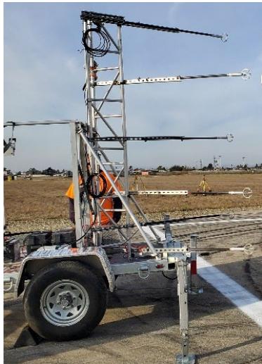
Figure 3. Vertical Array Mobile Cart

The sensor array reached a height of 10 ft above the grade of the test surface. The six Anemoment TriSonica 100 Hz Sphere Wind Flux Sensors mounted to the modified antenna array sampled at 100 Hz and output at 40 Hz. The sensors were located at 2, 3, 4, 6, 8, and 10 ft above the grade of the test surface. Square metal tubing was attached to the mast, and the sensors were mounted to carbon fiber tubes that were then mounted to the metal tubing, which allowed the sensors to telescope out.

3.3 AMBIENT ANEMOMETER

A single TriSonica 40 Hz Mini Sensor was deployed to monitor local wind conditions at the survey area. The reference anemometer was mounted on the same platform type as the horizontal sensors and at the same height but output at a rate of 1 Hz.

3.4 DATA ACQUISITION SYSTEM

The anemometers were directly connected to LI-COR Anemoment LI-570-4 data loggers with RS-232 cables. The data loggers were then connected to conventional laptops collecting and displaying the ASCII files from the logger locally. The data loggers also contained SD cards, which provided redundancy in data storage. All cables along the ground were weighted, taped, and/or staked down depending on the survey location.

4. SCOPE OF TEST

The DWOW surveys were conducted at various times and locations under daylight, visual meteorological conditions. DWOW data were collected at each anemometer location described in the horizontal sensor array and/or vertical sensor array associated with each survey discussed in Section 6. The pilots of the aircraft performed several preset maneuvers based on their and the OEM’s capability and risk tolerance. At the time of testing, aircraft flight profiles were limited due to the experimental nature of the aircraft and their early stage of development.

5. METHODOLOGY

A TLOF and vertiport symbol were painted per EB 105. A FATO was painted with a 6-inch line. The UTC time determined by the Global Position System (GPS) was noted during critical times of the flights for synchronization with modeling. The tolerances given to the pilot for the tests are shown in Table 4.

Table 4. Pilot Flight Tolerances

Roll	Pitch	Yaw	AGLHeight	Latitude/Longitude
$\pm 2 ^ { \circ }$	$\pm 2 ^ { \circ }$	$\pm 2 ^ { \circ }$	±2 ft	±2°ft

The dataset was processed through $\mathbf { M A T L A B } ^ { \textregistered }$ but not de-spiked for outliers. In certain industries, outliers are removed from datasets if they could be caused by instrument error from the ultrasonic anemometer because of various factors (e.g., radio frequency interference, acoustical interference, dust or water particles interrupting the sonic path). To remove outliers, one must assume that the unreal spikes in the series can be identified. However, anomalous values could be a result of real DWOW turbulence. De-spiking the data in the

present research was not performed in part due to the difficulty in determining false outliers from true outliers in such a turbulent environment. “One major problem with evaluating the performance of a data cleaning algorithm is that outside of obviously unphysical values, one cannot know a priori how incorrect a given set of data is” (Starkenburg et al., 2016). The variability of the vertical and horizontal direction of the DWOW in the present study is unpredictable1 and “the interactions between the wakes of the rotors are the prime reason why aircraft with eVTOL-like configuration tend to produce an outwash field that is particularly complex and spatially non-uniform in structure” (Brown, 2023). Brown (2023) warns that, even in simulation, there is a risk for “the velocities within the outwash [to be] mischaracterized, not only in terms of their spatial distribution but also very likely in terms of their magnitude as well as their inherent variation over time.” The researchers of this study believe it is inappropriate to try to de-spike the data at this time because of their unpredictability compared to other datasets where de-spiking is routine. Any smoothing comes in the use of the statistics described in the following paragraph.

MATLAB was used to process the datasets output from the data loggers. Table 5 presents a legend for the summarized descriptive statistics used. This research is limited by the finite number of sensor locations and heights surveyed during the flights. It is also limited by being conducted in a real-world environment where time with the aircraft and ambient conditions could not be controlled. While effort was taken to identify the best sensor locations to record the highest velocity using VVPM and changing the headings and altitudes of the aircraft during the maneuvers, different sensor locations or heights might have produced a different outcome. The nature of the dataset is turbulent, and thus it naturally includes peaks and valleys. To neither subdue nor smooth variability or give excessive meaning to individual measurements, descriptive statistics are included for both the entire dataset and for subsets of the dataset. The subset statistics include moving mean (average), standard deviation, and 95th percentile based on a 3-second time frame. Because a normal distribution cannot be guaranteed for every 3-second interval, the 95th percentile may be preferred over the standard deviation when considering outliers.

Table 5. Data Summary Statistics Legend

MM	3-Second Moving Mean (Average)
Max	Maximum
Max 3-s MM	Maximum 3-Second Moving Mean
Max 3-sMM+2MSD	Maximum 3-Second Moving Mean + 2 Moving StandardDeviations
Max 3-s M95%	Maximum 3-Second Moving 95th Percentile (3-second)

The survey measurements for the eVTOL aircraft included in the research are compared to VVPM modeling and simulation where possible. This was done to determine the ability to use the VVPM method for simulating the DWOW of eVTOL aircraft in different operational scenarios in the future.

6. RESULTS

This section covers the results from the DWOW surveys.

6.1 eVTOL #1

The aircraft was remotely piloted. All headings for this set of surveys are referenced to magnetic north. The sensors were located on radials 290°, 200°, 110°, and 20° except for three, which were positioned at 50°, 65°, and 165° to allow room for aircraft to taxi between sensors and to increase the number of sensors in the quartering quadrants to reflect OEMconducted modeling of their aircraft’s DWOW. The sensor distances from the center of the TLOF are shown in Table 6.

Table 6. eVTOL #1 Sensor Labels and Distances

Sensor Name	Type	Distance fromTLOF(ft)
N-1-S	Sphere	33
N-5-M	Mini	46
N-9-M	Mini	69
E-2-S	Sphere	23
E-6-M	Mini	46
E-10-M	Mini	69
S-3-S	Sphere	23
S-7-M	Mini	46
S-11-M	Mini	69
W-4-S	Sphere	23
W-8-M	Mini	46
W-12-M	Mini	69
NE-13-S	Sphere	28
SE-14-S	Sphere	28

Note: S in sensor name denotes it as a Sphere, while M in the sensor name denotes it as a Mini.

The remote pilot of the aircraft conducted four flights that included 3-ft and 10-ft hovers and 10-ft departures and arrivals for a total of four DWOW surveys. These flights are detailed in Table 7.

Table 7. eVTOL #1 Flight Details for Each Survey

Survey #	Height (ft AGL)	Target Magnetic Heading
S1—Hover (takeoff within sensors) Liftoff 290°
1.1	NA—Takeoff within sensors	290°
1.2	3	290°
1.3	3	245°
1.4	3	200°
1.5	3	155°
1.6	3	110
S1—Hover (takeoff within sensors) Liftoff 290°
1.7	3	65°
1.8	10	290°
1.9	10	245°
1.10	10	200°
1.11	10	155°
1.12	10	110°
1.13	10	65°
1.14	NA—Land within sensors	290°
S2--10-ft AGL Departure (takeoff within sensors) Liftoff 290°
2.1	10	290°
	NA—Land outside sensors
S3—10-ft AGL Departure (takeoff within sensors) Liftoff 290°
3.1	10	290°
[	NA—Land outside sensors
S4—10-ft AGL Approach, Hover, Touchdown (takeoff outside sensors)		ctakeoff outside sensors)
4.1	10	290°
4.2	10	245°
4.3	10	200°
4.4	10	155°
4.5	10	110°
4.6	10	65°
4.7	10	290°
4.8	NA—Land within sensors	290°

Post-test analysis revealed that the data logger receiving signals from sensor N-5 had an unattached wire to a port not in use during Survey 2. This wire caused sporadic noise for N-5 as it shared the same bus. This noise occurred during Survey 2 and affected the moving mean, standard deviation, and 95th percentile on this sensor, so it was removed from the maximum statistics for all surveys shown in the next section. Post-test analysis also revealed that the data loggers receiving signals from Sensors NE-13, S-3, S-7, and S-11 were recording at 20 Hz while all others were recording at 40 Hz. Additionally, Survey 4 sensor NE-13 disconnected from the data logger due to DWOW impact from the aircraft and stopped recording data partway through the test. There is also a very short gap in data in Survey 1 on the datalogger that affects Sensors E-2, E-6, and E-10. The results from these sensors during these surveys are included in statistics but the maximum results might have been higher had these gaps not existed. Regarding flight tracks, the pilot of the aircraft was asked to maintain the flight test tolerances in Table 4; however, those tolerances were not verified.

6.1.1 eVTOL #1 Horizontal Array Velocity Results

Figure 4 shows the sensor locations as depicted on the landing area in a plan view and includes the maximum measurements at each sensor across all the surveys. Table 8 shows the same but in tabular view and sorted by distance from the TLOF center. Figure 5 provides more detail by graphing the maximum readings at each sensor location for each survey (sorted by sensor distance from TLOF).

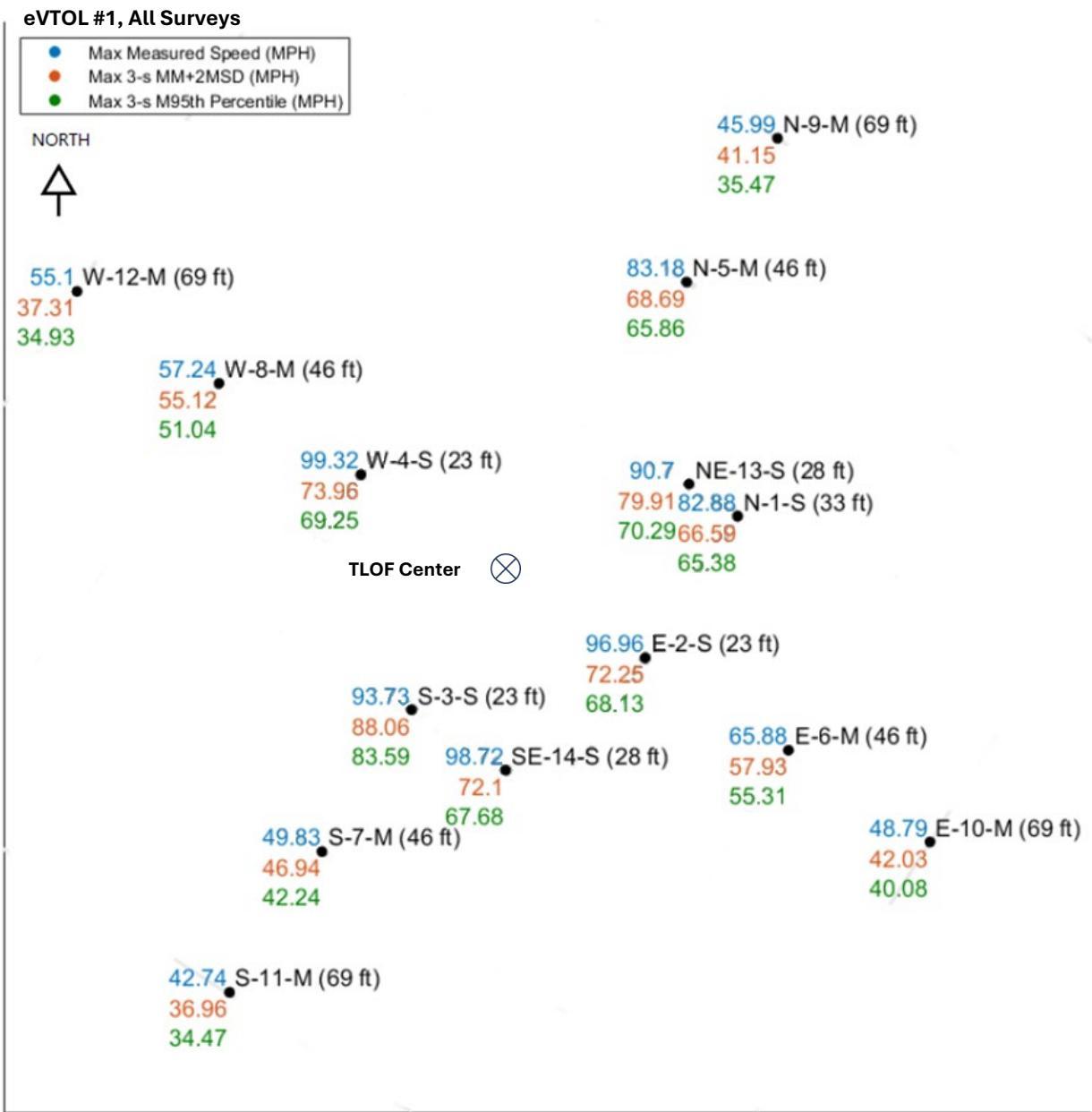
NOTE: The statistics shown are independent of each other. The maximums for any one sensor or specific statistic may not come from the same time window or the same survey.

Figure 4. eVTOL #1 Maximum Velocity Recorded at Each Sensor Across All Surveys in Plan View
Table 8. eVTOL #1 Maximum Velocity Recorded at Each Sensor Across All Surveys

Sensor ID	Distancefrom TLOFCenter (ft)	Max	Max 3-sMM	Max 3-s MM+2MSD	MaxM95%
N-1-S	33	82.88	42.86	66.59	65.38
N-5-M	46	83.18	38.09	68.69	65.86
N-9-M	69	45.99	25.93	41.15	35.47
E-2-S	23	96.96	44.50	72.25	68.13
E-6-M	46	65.88	36.57	57.93	55.31
E-10-M	69	48.79	26.46	42.03	40.08

Sensor ID	Distancefrom TLOFCenter (ft)	Max	Max 3-sMM	Max 3-s MM+2MSD	MaxM95%
S-3-S	23	93.73	50.09	88.06	83.59
S-7-M	46	49.83	26.65	46.94	42.24
S-11-M	69	42.74	21.47	36.96	34.47
W-4-S	23	99.32	44.94	73.96	69.25
W-8-M	46	57.24	36.34	55.12	51.04
W-12-M	69	55.10	23.92	37.31	34.93
NE-13-S	28	90.70	44.98	79.91	70.29
SE-14-S	28	98.72	45.39	72.10	67.68

NOTE: The statistics shown are independent of each other. The maximums for any one sensor or specific statistic may not come from the same time window or the same survey.

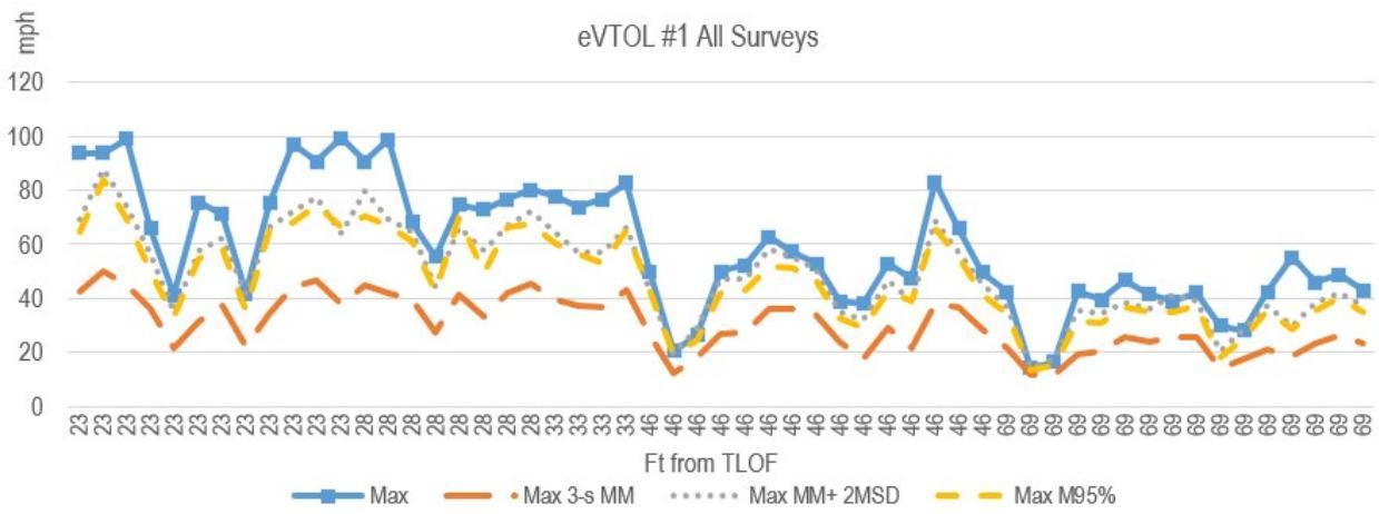
Figure 5. eVTOL #1 Line Graph of Maximum Velocity Recorded at Each Sensor for Each Survey (Sorted by Distance from TLOF Center from Left to Right)

6.1.2 eVTOL #1 Comparison to VVPM Modeling and Simulation

The eVTOL #1 was the first aircraft to be modeled with VVPM and simulated, so it provided the first feedback regarding the DWOW velocity predictions from VVPM. The figures that follow show a snapshot of the total velocities at 23, 46, and 69 ft from the TLOF. The color contour maps are for one-time frame in a video animation of the total velocity shown via color contour plot. The x-axis shows the lateral aircraft axis for the frontal view and the yaxis shows the height above the ground. A scale on the right associates colors to total velocity magnitudes. As shown in Figure 6, close to the aircraft, at 23 ft from the TLOF center, significant total velocities (red-yellow color) are visible. The section cut is close to the front propellers. The high-velocity contours in Figure 6 are, therefore, dominated by downwash. Farther away at 46 ft from the TLOF center, as shown in Figure 7, the velocity concentrations of outwash close to the ground and recirculation is higher above the ground. One can observe the directionality of the outwash by the distinct color (red-yellow) concentrations. There are also blue areas where ground sensors measure low outwash velocities.

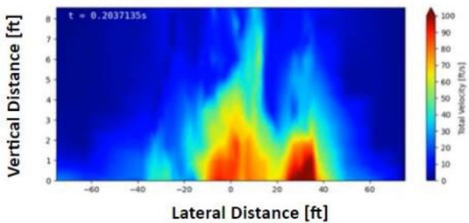
Figure 6. eVTOL #1 Modeled Total Velocity at 23 ft

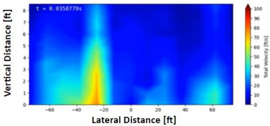
Figure 7. eVTOL #1 Modeled Total Velocity at 46 ft

Figure 8 shows the predicted outwash (total) velocities at the safety area boundary. Measured data indicate high outwash velocities at and above 27.3 mph (40 ft/s). The color contour map shows low total velocities at the vertical plane except for one small area on the very right and low to the ground. The predicted position of the higher velocity outwash did not coincide with the actual measurement location in the test, which was in the blue-colored area. In addition, it was observed that, far from the aircraft, the propeller wake was very turbulent, which resulted in the peak velocities continuously shifting over time.

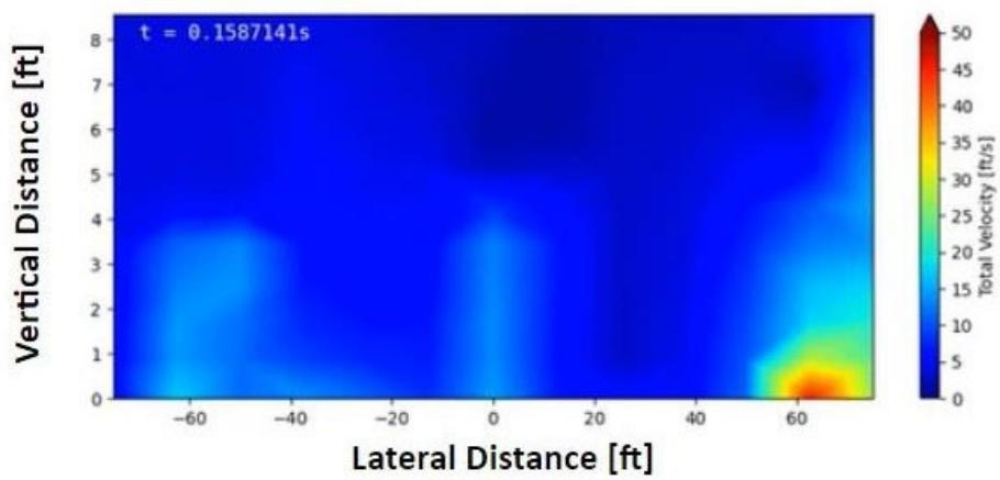
Figure 8. eVTOL #1 Modeled Total Velocity at 69 ft

The survey conditions were not well suited for comparison because the vertical sensor array was not included, the aircraft positions were not consistently held, and the ambient wind conditions varied throughout the survey. However, an important observation was made during the test and post-processing of the measured data. The outwash airspeed for sensors at the outer boundary of the safety area showed higher magnitudes than had initially been predicted by VVPM. A detailed review of the results showed that viscous vortex particles were retired too early in the VVPM simulation due to the limited GPU memory available at that time. Particles are continuously created at the trailing edge of the propeller blades during simulation and travel with the wake away from the aircraft. The particles are retired based on both wake time and distance traveled since initiation. The longer the minimum wake time/distance traveled, the more particles are covered in the simulation, which require more GPU memory. Because VVPM memory usage is a combination of simulation fidelity (emitted particle per blade span), total number of propeller blades, simulation duration, and life of particles, compromises have to be made in some cases, and thus particles were retired too early for the far field locations. The life of these particles was extended to the physical limits of the hardware (graphics card memory), which included the ability to track approximately 4.5 million particles at the time of the simulations. Ultimately, results showed that the available graphics card memory might adversely impact simulation fidelity of eVTOL configurations with a large number of propeller blades compared to helicopters.

6.2 eVTOL #2

The aircraft was autonomously piloted. The horizontal sensors were located on radials of 333°, 153°, and 108° (referenced to true north). The vertical sensor array was approximately 26 ft behind the aircraft in the right rear quadrant. The sensor distances from the center of the TLOF are shown in Table 9.

Table 9. eVTOL #2 Sensor Labels and Distances

Horizontal ArraySensor Name	Azimuth fromTLOF Center	Distance fromTLOF Center (ft)
A10-S-A2	153°	38
A20-S-A2	153°	50
A30-S-A2	153°	58
A40-M-A1	153°	75

Horizontal ArraySensor Name	Azimuth fromTLOF Center	Distance fromTLOF Center (ft)
A50-M-A1	153°	85
A60-M-A1	153°	95
B10-S-B2	333°	37
B20-S-B2	333°	50
B30-S-B2	333°	58
B40-M-B1	333°	75
B50-M-B1	333°	85
B60-M-B1	333°	95
C10-S-C2	108°	53
C20-S-C2	108°	71
C30-S-C2	108°	82
C40-M-C1	108°	106
C50-M-C1	108°	116
C60-M-C1	108°	126
Vertical SensorName	Azimuth fromTLOF Center	Distance fromTLOF Center (ft) /(ft AGL)
A10-S-A2	229°	26/2
A20-S-A2	238°	24/3
A30-S-A2	229°	26/4
B10-S-B2	238°	24/6
B20-S-B2	229°	26/8
B30-S-B2	238°	24/ 10

Note: S in sensor name denotes it as a Sphere while M in the sensor name denotes it as a Mini.

The aircraft flew six autonomous flights and one set of tethered engine run-ups. These flights are detailed in Table 10. The horizontal sensors were removed and six of them were placed on the mobile cart for Survey 7, which included three engine runups to a point where the aircraft would have become airborne had it not been tethered.

Table 10. eVTOL #2 Flight Details for Each Survey

Survey #	Outbound	Inbound
1	333°	153°
2	18°	198°
3	63°	243°
4	108°	288°
5	153°	333°
6 (Hover)	153°	NA
7a (Tethered)	84°	NA
7b (Tethered)	84°	NA
7c (Tethered)	84°	NA

Post-test analysis revealed that the GPS unit that receives the timestamp for one of the dataloggers failed during Survey 4 and Survey 5. Therefore, the timestamps associated with

C40, C50, and C60 sensors are assumed and were created based on a comparison of the signal events from another sensor (A60) that was a comparable distance from the TLOF. On Survey 6, a GPS unit also failed, this time recording the same timestamp partway through the survey to the end. This affected C10 and C20, so these timestamps are also assumed and were created using the same process used for Surveys 4 and 5. These failures did not affect the wind characteristics data received from the sensors. Post-test analysis also revealed that the ambient sensor did not collect data during the Survey 7 series.

Post-test analysis of the aircraft navigational data received from the OEM revealed that it was not of high enough fidelity to show the aircraft track and altitude. While the temporal resolution of the data stream is good, 100 Hz, and the elevation resolution is sufficient at 4 decimal places, the latitudes and longitudes have been truncated to four decimal places.

6.2.1 eVtOL #2 Horizontal Array Velocity Results

Figure 9 shows the sensor locations as depicted on the landing area in a plan view and includes the maximum readings at each sensor across all the surveys. Table 11 shows the same but in tabular view. Figure 10 provides more detail by graphing the maximum readings at each sensor location for each survey (sorted by sensor distance from TLOF). Note that Survey 7 did not include the horizontal array, so those sensors are not included in either the table or graphs.

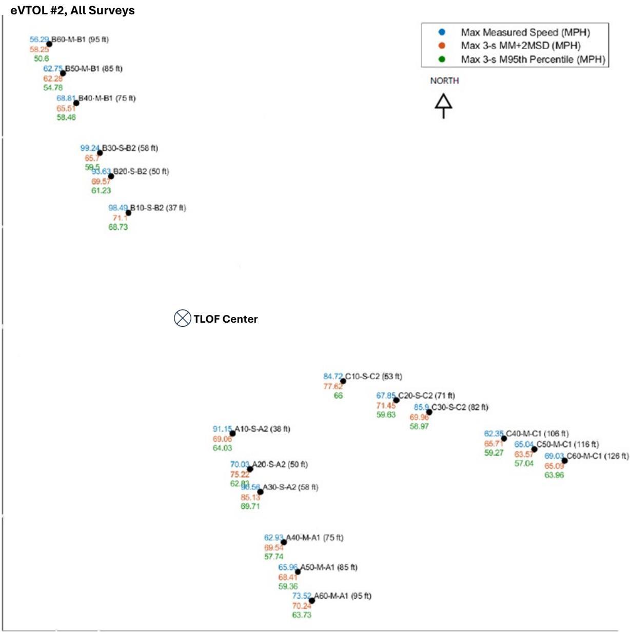
NOTE: The statistics shown are independent of each other. The maximums for any one sensor or specific statistic may not come from the same time window or the same survey.

Figure 9. eVTOL #2 Maximum Velocity Recorded at Each Sensor Across all Surveys in Plan View

Table 11. eVTOL #2 Maximum Velocity (mph) Recorded at Each Sensor Across All Surveys

HorizontalArray SensorID	DistancefromTLOFCenter (ft)	Max	Max 3-sMM	Max 3-sMM+2MSD	Max 3-sM95%
A10-S-A2	38	91.15	39.11	69.06	64.03
A20-S-A2	50	70.03	42.44	75.22	62.83
A30-S-A2	58	90.56	46.81	85.13	69.71
A40-M-A1	75	62.93	37.28	69.54	57.74
A50-M-A1	85	65.96	36.79	68.41	59.36
A60-M-A1	95	73.52	41.33	70.24	63.73
B10-S-B2	37	98.49	49.58	71.10	68.73
B20-S-B2	50	93.63	47.26	69.57	61.23
B30-S-B2	58	99.24	44.85	65.70	59.50
B40-M-B1	75	68.81	42.41	65.51	58.46
B50-M-B1	85	62.75	40.73	62.28	54.78
B60-M-B1	95	56.29	38.59	58.25	50.60
C10-S-C2	53	84.72	44.87	77.62	66.00
C20-S-C2	71	67.85	41.20	71.45	59.63
C30-S-C2	82	85.90	40.92	69.96	58.97
C40-M-C1	106	62.35	37.65	65.71	59.27
C50-M-C1	116	65.04	36.43	63.57	57.04
C60-M-C1	126	69.03	38.78	65.09	63.96

NOTE: The statistics shown are independent of each other. The maximums for any one sensor or specific statistic may not come from the same time window or the same survey.

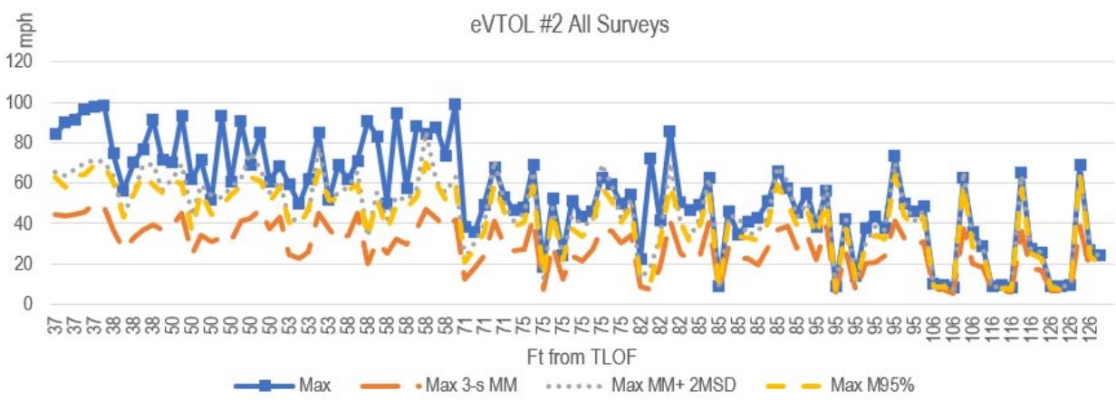
Figure 10. eVTOL #2 Line Graph of Maximum Velocity (mph) Recorded at Each Sensor for Each Survey (Sorted by Distance from TLOF Center from Left to Right)
6.2.2 eVTOL #2 Vertical Array Velocity Results

Table 12 shows the maximum recordings for the vertical array. Note this array was only used when the aircraft was tethered (Surveys 7A, 7B, and 7C) with sensors from the horizontal array mounted on the mobile cart. Therefore, there are no horizontal array sensors used in Surveys 7A, 7B, or 7C.

Table 12. eVTOL #2 Maximum Velocity (mph) Recorded for All Surveys

VerticalArray SensorID	AGL (ft)	Max	Max 3-sMM	Max 3-sMM+2MSD	Max 3-sM95%
A10-S-A2	2	96.52	49.43	78.76	80.11
A20-S-A2	3	94.59	34.66	57.91	56.20
A30-S-A2	4	92.85	41.84	71.39	68.56
B10-S-B2	6	81.63	31.56	62.58	58.98
B20-S-B2	8	61.86	24.07	48.82	49.17
B30-S-B2	10	53.19	24.42	40.17	38.49

NOTE: The statistics shown are independent of each other. The maximums for any one sensor or specific statistic may not come from the same time window or the same survey.

6.2.3 eVTOL #2 Comparison to VVPM Modeling and Simulation

The computational cost, including the GPU memory usage, for VVPM simulation is proportional to the total number of blades, which, as with eVTOL #1, proved to be challenging for this VVPM simulation. A reduction of the computational cost was achieved by reducing the number of blades per propulsion but keeping it aerodynamically equivalent. The model was rigorously scaled to reflect the original propeller aerodynamic performance to improve the accuracy of DWOW calculation.

The manufacturer did not provide geometric aircraft data for the propeller blade planforms and propeller hub locations to aid the development of the simulation model. The eVTOL #2 FLIGHTLAB/VVPM simulation model was therefore created based on public domain data and the modeling team’s best practices. The simulation validation focused on steady-state flight test points from the hover ladder and tethered flight to improve the setup of the VVPM DWOW flow field simulation with initial test conditions matching the flight test data. For the hover ladder, for example, the FLIGHTLAB model was trimmed at the measured heights above the ground, providing a solution for the individual propeller speeds which could be compared to recorded aircraft data. The difference between simulation and flight test records reflected the uncertainties with the aircraft modeling properties (e.g., propeller blade geometric planform, position) The propeller speed was constant in the VVPM simulations while the original aircraft in the flight test used small variations of propeller speed in the flight control system to maintain hover position and aircraft attitudes. Note also that the blockage effects from the aircraft surfaces were not included in the VVPM simulation.

Exploratory DWOW simulation of steady hover at several wheel/skid heights above the ground showed significant propeller-on-propeller and propeller wake interactions. These interactions lead to significant upwash between propellers and pronounced propeller wake unsteadiness that did not match video documentation of the aircraft during flight testing, which displayed very controlled aircraft position and attitudes. An in-depth investigation identified noticeable blade stall, which typically does not occur on well-designed lift propellers for eVTOL aircraft. The modeling team, which has experience in rotor/propeller design, created an improved blade twist and chord distributions to overcome the lack of data from the manufacturer. The resulting propeller designs exhibited a reasonable wake profile. The design exercise provided additional insight into the relationship between simulation model properties and the accuracy of predicting the overall aircraft DWOW flow field. This relationship is dependent on aircraft configuration, with some eVTOL configurations (i.e., configurations with propellers in proximity of each other and adjacent aircraft structures) requiring detailed OEM propeller geometric properties to develop a reasonable propeller model for the VVPM DWOW simulation.

When the aircraft model is based on geometric, inertial, and aerodynamic properties from the manufacturer, the recorded aircraft control parameters (e.g., propeller rotational speeds, collective blade pitch, control surface deflections) from the flight survey data can be “replayed” (sometimes with minor adjustments) in the simulation, thus leading to closely matching the aircraft response and achieving good correlation. Matching the operation of the original aircraft in simulation, in turn, improves the DWOW wake predictions and correlation with measured data for simulation validation.

6.2.3.1 Survey 6—Hover 11-ft Wheel/Skid Height Validation

The first simulation validation test case was conducted in hover at an 11-ft wheel/skid height above the ground and was part of Survey 6. The sensor names from the survey are also shown in Figure 9. Most sensors are within the VVPM wake. Some outfield sensors were not reached by the VVPM wake as the vortex particles retired from the simulation due to hardware memory constraints. Approximately 6 million particles were released into the simulation domain, which is presently the largest number of particles in any of modeling team’s VVPM simulations.

The time history of total vertical thrust (lift) of all propellers for approximately 30 revolutions, or a 1.3-second simulation time, was reviewed, and the mean of the thrust matched the vehicle gross weight as is expected in hover. There were small amplitude oscillations caused by the unsteadiness of the wake and due to aerodynamic interactions, which have no significant effect on the aircraft vertical position given their magnitude and frequency and the aircraft inertia. A preliminary review of the measured velocities from the horizontal sensor array indicated the presence of significant flow unsteadiness. Although the airspeed sensors in the horizontal measurement array were located 3 ft above ground, the VVPM simulation was set up with additional vertical sampling points ranging from 2 ft to 6 ft and with increments of 0.2 ft at the horizontal sensor array locations. This was done to better understand the vertical variations of local DWOW velocities at the position of the sensors in this survey. Note that the mean ambient wind was subtracted from the survey results to properly correlate with the VVPM simulation.

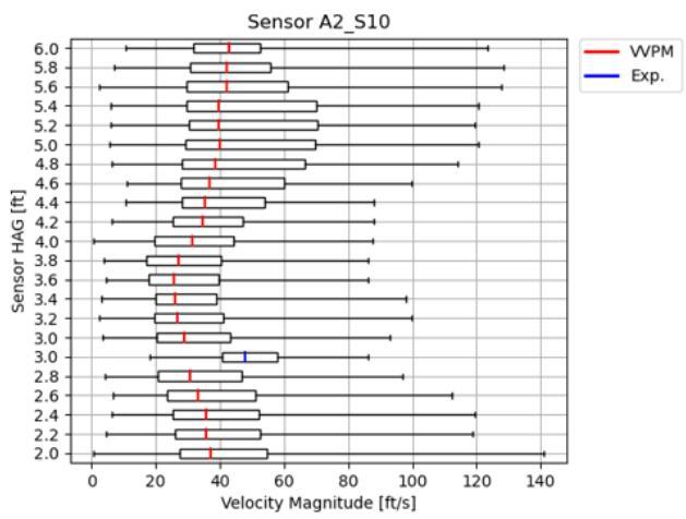
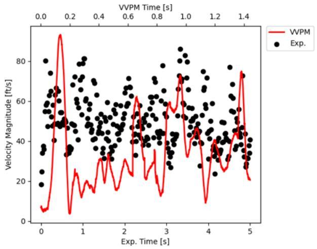
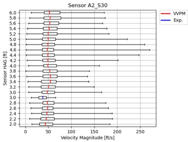
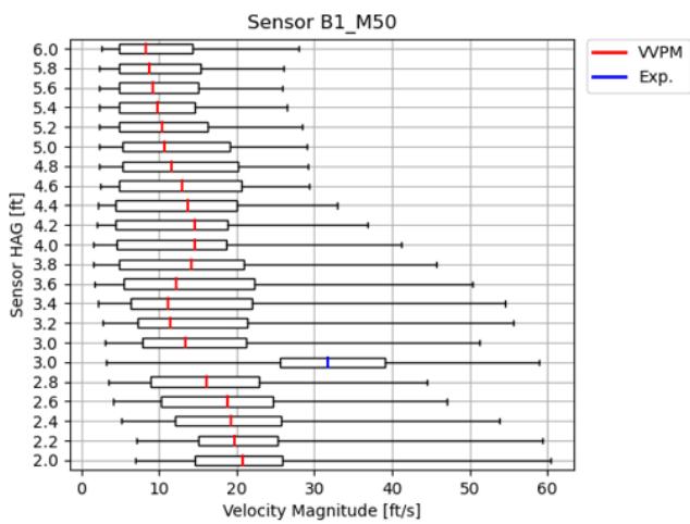
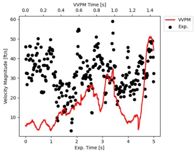
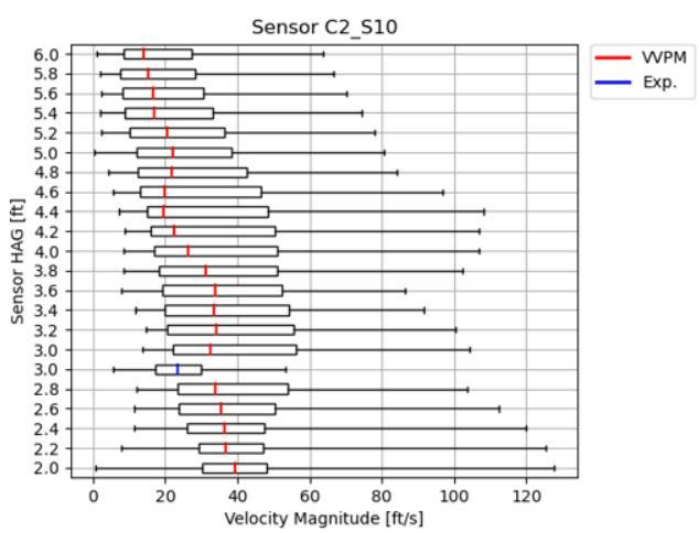
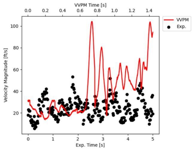
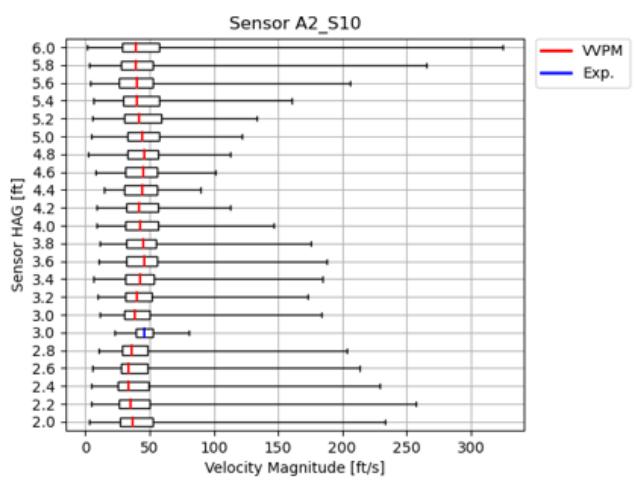
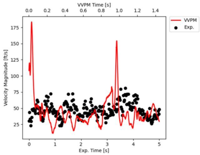
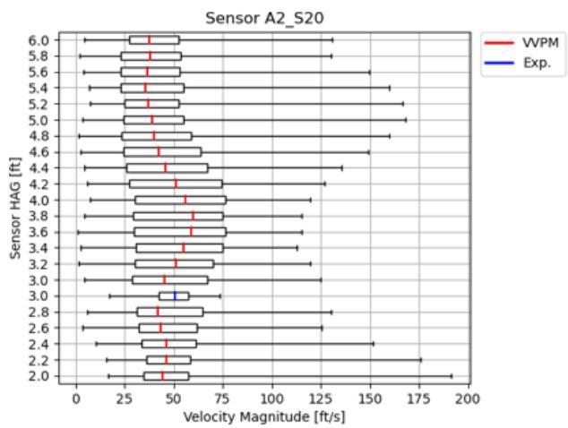
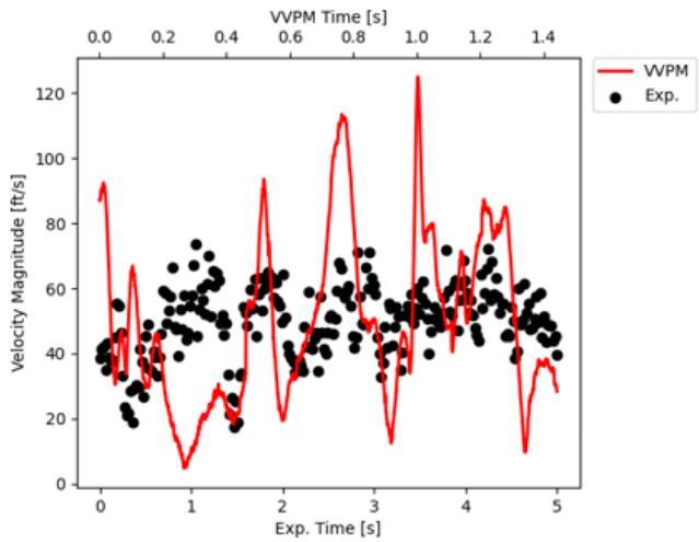
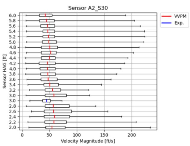
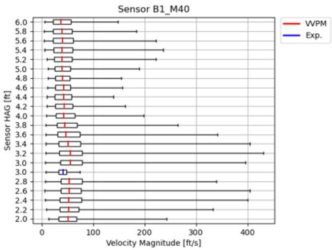
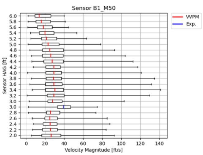
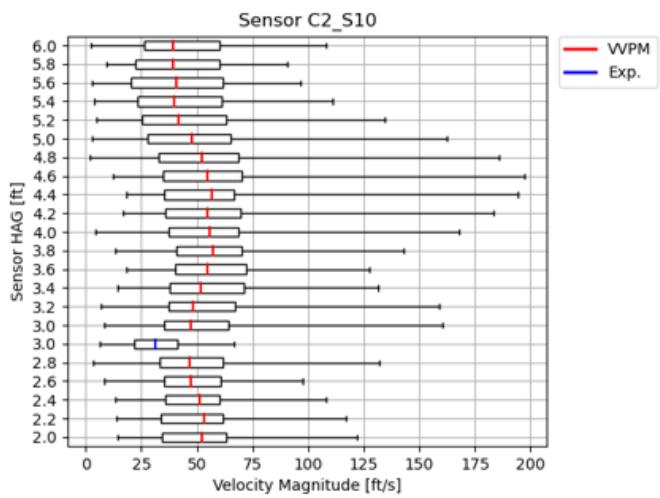
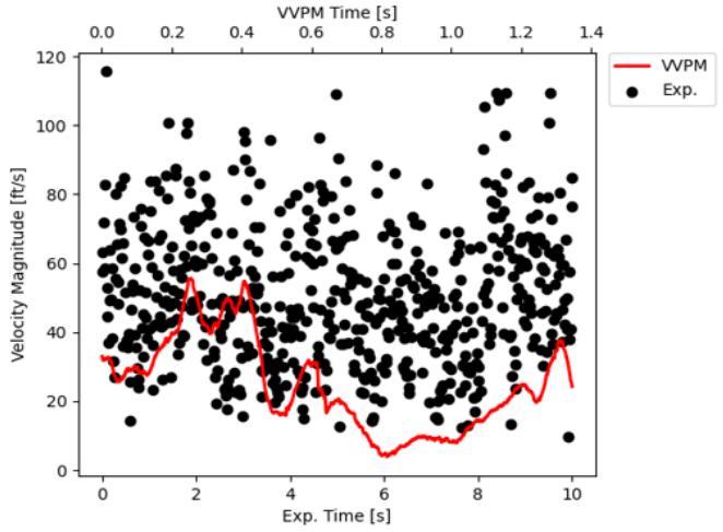
Figures 11 through 16 show the comparison of the velocity magnitude from VVPM simulation and measurements for sensors A2-S10, A2-S20, A2-S30, B1-M40, B1-M50, and C2-S10. Simulation velocity magnitude predictions are recorded for 30 propeller revolutions, or approximately 1.3 seconds. The results for each sensor show a statistical analysis as a boxplot diagram on the left and the time histories of the velocity magnitudes on the right. The vertical axis of the box plot charts shows the vertical position of the simulation sampling points (red median line) and the original sensor (blue median line) at 3 ft. Boxplots display 50% of the data inside the box with a vertical line (red/blue) annotating the median of all the data in the set. The whiskers of the box plot contain the lower/upper 25% of data and include the minimum and maximum values. The x-axis of the box plot charts is the velocity magnitude in feet per second. Consequently, the size of the box and the range of the whiskers with respect to the x-axis provide a visual indication of the unsteadiness of the flow. The overlap of the box for the measured data (blue median line of experimental data) at 3 ft above the ground with the adjacent simulation sampling points provides an insight into the correlation between measurements and simulation predictions. The agreement of the blue median line (measurement/experiment) with the adjacent red median lines of the simulation predictions is also an indicator for the accuracy of the correlation. Furthermore, the unsteadiness measured in flight and predicted by simulation must also be considered when assessing the correlation between measurements and simulation predictions.

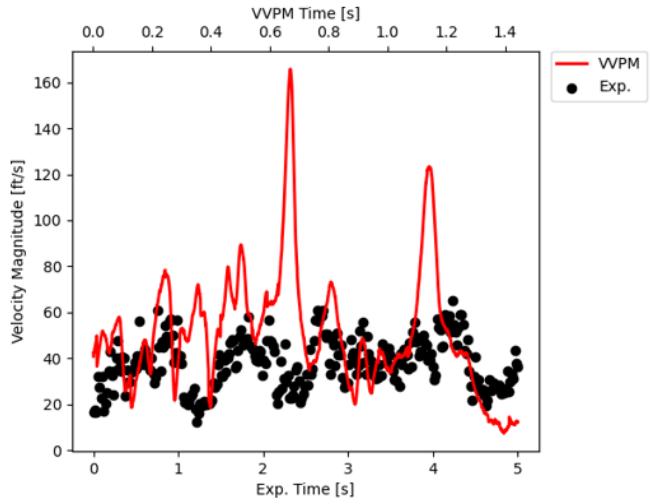
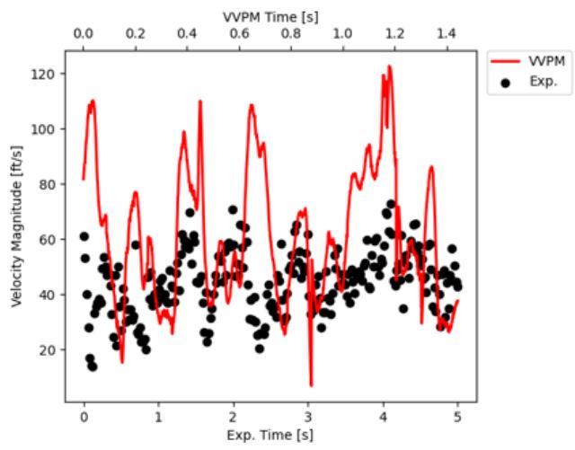
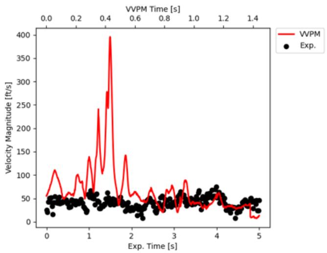
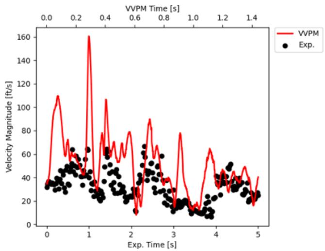
The time histories on the right side in Figures 11 through 16 show the simulation predictions as a continuous red line and the measurements (experiments) as solid black circles. The xaxis shows the elapsed time, and the y-axis shows the velocity magnitude. The time history plots are evaluated in conjunction with the box plots providing an additional visualization of the correlation between measured and predicted local velocities. The time history plot shows exclusively the simulation at the vertical location of the sensor (3 ft); the other sampling points (as shown in the box plot) were omitted.

(a) Boxplot of Velocity Magnitude

(b) Time History of Velocity

Figure 11. Velocity Predictions at Sensor A2-S10

(a) Boxplot of Velocity Magnitude

(b) Time History of Velocity
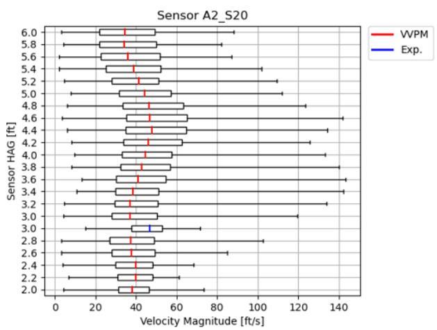
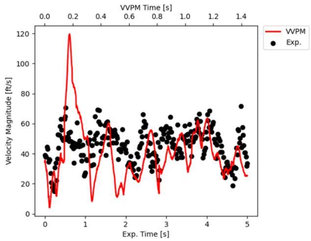
Figure 12. Velocity Predictions at Sensor A2-S20

(a) Boxplot of Velocity Magnitude

(b) Time History of Velocity

Figure 13. Velocity Predictions at Sensor A2-S30

(a) Boxplot of Velocity Magnitude

(b) Time History of Velocity
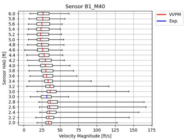
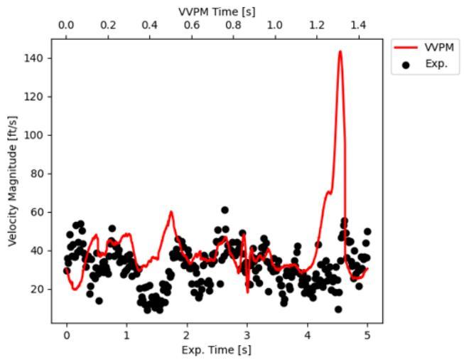
Figure 14. Velocity Predictions at Sensor B1-M40

(a) Boxplot of Velocity Magnitude

(b) Time History of Velocity

Figure 15. Velocity Predictions at Sensor B1-M50

(a) Boxplot of Velocity Magnitude

(b) Time History of Velocity
Figure 16. Velocity Predictions at Sensor C2-S10

Figures 12, 13, and 14 show a limited correlation between simulation predictions and measured data. Note that the simulation was run at a much higher sampling rate than the measured data and, therefore, not all peaks should be expected to be reflected in the measured data. Figures 11 and 15 show even less correlation as observed for the other sensor locations. In Figure 15 (sensor B1-M50) for example, the measured velocity was significantly larger than predicted by simulation. This is confirmed in both the box plot and the time history. The unsteadiness of the velocity magnitude (size of box and range of whiskers) matches well.

Investigations were focused on the sensor locations that had lower correlation. For outboard sensors, the predictions fall in the lower part of measured data range. For those sensors, the simulated wake domain might not have fully covered them due to GPU memory constraint. After the vortex particles are shed from propeller blades, they are retired based on the

maximum wake age that defines the size of the VVPM simulation domain where vortex particles can reach. The specification of the wake age is constrained by the available GPU card memory. Thus, near the wake boundary, as affected by the maximum wake age set by VVPM simulation, the prediction can be in the lower part of measured data range, but still within the data scatter range. Conversely, horizontal measurement locations close to the lift propellers are affected most by some of the uncertainties in the aircraft modeling properties (e.g., propeller blade planform).

The vertical variation of the flow sampling points at the horizontal location of specific sensors provided additional insight into the velocity magnitude profile as a function of height above the ground. For sensor B1-M40 in Figure 14, the vertical velocity magnitude from VVPM simulation confirms that the sensor measured the maximum velocity magnitude at this horizontal location even though the simulation slightly overpredicted velocity magnitudes. Conversely, for sensor A2-S20 in Figure 12, simulation predicted the maximum velocity magnitude at 3.6 ft above the ground possibly due to the proximity to a lift propeller and, therefore, a higher downwash component.

6.2.3.2 Survey #6—Hover 22 ft. Wheel/Skid Height Validation

This hover test point was conducted at a 22-ft wheel/skid height above the ground. Comparing the time histories of the total propeller thrust between the 11- and 22-ft hover heights shows less variation of the mean thrust and smaller variation magnitude and unsteadiness for the 22-ft height case. This confirms the previously stated observation of aircraft unsteadiness at lower hover heights, especially below 10 ft above the ground.

(a) Boxplot of Velocity Magnitude

(b) Time History of Velocity
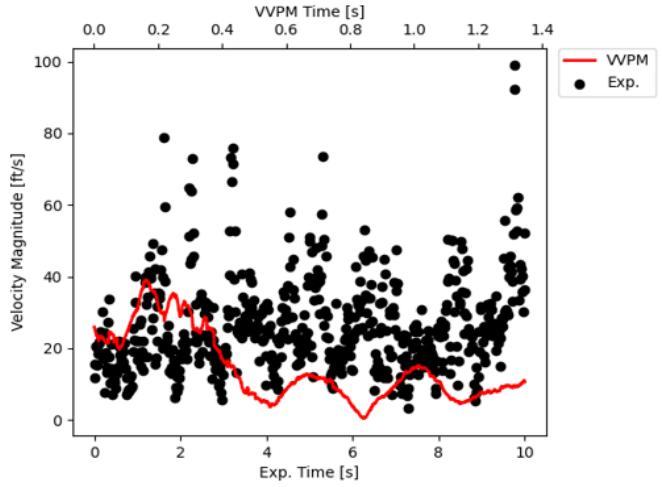
Figure 17. Velocity Predictions at Sensor A2-S10

(a) Boxplot of Velocity Magnitude

(b) Time History of Velocity

Figure 18. Velocity Predictions at Sensor A2-S20

(a) Boxplot of Velocity Magnitude

(b) Time History of Velocity
Figure 19. Velocity Predictions at Sensor A2-S30

(a) Boxplot of Velocity Magnitude

(b) Time History of Velocity

Figure 20. Velocity Predictions at Sensor B1-M40

(a) Boxplot of Velocity Magnitude

(b) Time History of Velocity
Figure 21. Velocity Predictions at Sensor B1-M50

(a) Boxplot of Velocity Magnitude

(b) Time History of Velocity
Figure 22. Velocity Predictions at Sensor C2-S10

In a qualitative comparison of the correlation of velocity magnitude predictions between the 11- and 22-ft hover cases, comparing Figures 11 through 16 and Figures 17 through 22, the correlation of the velocity magnitude (median) seems better for the 22-ft hover case. The general observation made for the previous hover cases can be found again in the correlation for the 22-ft hover height case with some sensors matching better than others.

However, it is noticeable that in the 22-ft case, the simulation overpredicted the unsteadiness of the flow for almost all sensors. Comparing the time histories for the 22-ft hover height case, the red lines seem to show more outliers and excursions beyond measurements (black circles). Note also that a visual assessment is somewhat skewed because the scales of the xaxes of the box plots charts in Figure 17 through Figure 22 are different due to the magnitude of some outliers from flow simulation.

The observations on vertical variation are consistent for both 11- and 22-ft hover heights. The simulation results show a consistent vertical velocity magnitude profile, i.e., adding a line connecting all red median lines in the box plots.

Given the uncertainty in aircraft modeling properties and aircraft power/thrust state during the flight, the correlation between measured and predicted DWOW velocity magnitudes cannot be truly confirmed. Limitation on the range of VVPM predictions (e.g., reaching and exceeding the outfield sensor locations) was challenging but can further be improved with adjustment of particle emission resolution and new computing hardware. The GPU industry and market are currently experiencing rapid growth and improvement, mainly driven by the demands of computing needs for artificial intelligence and cryptocurrency.

6.2.3.3 Survey 7—Tethered Aircraft Test Validation

To use the vertical sensor array in close proximity to the aircraft, the aircraft was tethered to the ground to prevent it from drifting and contacting the sensor array. The vertical sensor array was situated at a horizontal position (horizontal distance and azimuth angle) from the aircraft. Although horizontal sensor locations varied somewhat, sensors were spaced

vertically and were, therefore, capable of measuring the vertical DWOW velocity profile at the horizontal location relative to the aircraft. Figure 23 shows the vertical flow sensor array with annotated sensor names and locations as used in the survey.

Typically, lift propeller rotational speeds on models using detailed aircraft properties from the manufacturer can be directly replayed (with small adjustments) in the simulation model to match the aircraft thrust with the original aircraft in the flight test. For this validation, however, the aircraft thrust level had to be estimated from aircraft measurements and previous validation cases. To estimate the aircraft total thrust, the recorded lift propeller rotational speeds in the tethered survey were compared with those from Survey 6, the hover ladder, knowing that in the hover ladder, the total lift propeller thrust was equivalent to the aircraft gross weight (a known entity). The propeller speeds indicated that the thrust in the tethered test exceeded the hover thrust. Thus, the tethers prevented aircraft takeoff and vertical climb. Applying the delta between propeller speeds from tethered and hover ladder aircraft data to the propeller speeds in the simulation model from the hover ladder, two thrust levels were simulated for the tethered survey case and to investigate the sensitivity of the total thrust uncertainty in the DWOW prediction.

Comparisons of the correlation of the velocity magnitudes for the hover and the elevated thrust cases showed very similar results. This report shows the results for the elevated thrust case (i.e., the thrust assumed to have been used in the actual survey). Figure 24 shows the statistical analysis results and comparison between measured and predicted data. The unsteadiness is also very similar between measurements and predictions (size of boxes in chart). However, the vertical array measurements included higher velocity magnitude outliers or peaks, symbolized by the whiskers. VVPM simulation shows fewer peak variations because the propellers operated at a constant speed in simulation, while the actual survey shows some variation in the recorded aircraft data. While the VVPM simulation shows a vertical velocity profile, i.e., when connecting the red median lines with a continuous vertical line, typical for a flow with a ground boundary layer (maximum velocity at approx. 2.54 ft), the measured data do not show such a consistent profile, which might indicate some aerodynamic interaction of the sensors with the supporting structure (e.g., obstructions, blockage, interference).

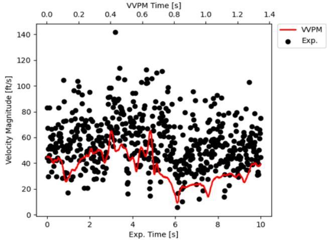
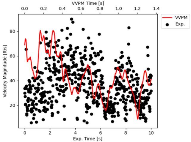
Figure 25 shows the time histories of the velocity magnitudes in the same format as previously discussed for the hover ladder validation cases. It shows the same results as discovered in the box plot in the time domain. The larger unsteadiness, especially the outliers, are this time visible in the measured data.

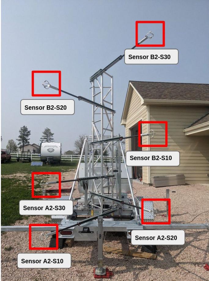
Figure 23. Vertical Array Sensor Configuration

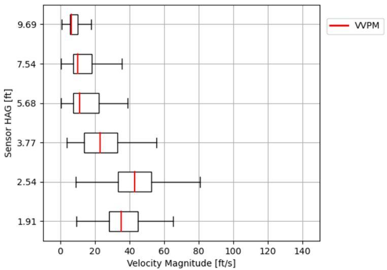
(a) Elevated Thrust Setting (VVPM Simulation)

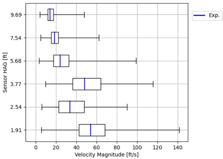
(b) Experimental Data
Figure 24. Tethered Test Case Correlation—Boxplots of Velocity Magnitude

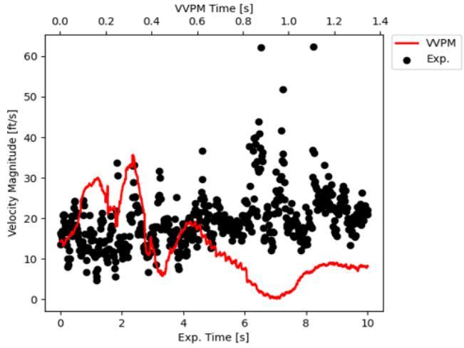
(a) Sensor A2-S10

(b) A2-S20

(c) Sensor A2-S30

(d) Sensor B2-S10

(e) B2-S20

(f) Sensor B2-S30
Figure 25. Tethered Test Case Correlation—Time Histories of Velocity of Magnitudes

The horizontal array included three rows (A, B, and C) with a total of 18 sensors. The OEM’s risk tolerance did not allow for flying near the vertical sensor array, so it was not used during this survey. The aircraft was flown with the pilot on board. The horizontal sensors were located on radials of 90°, 270°, and 225° (referenced to true north). The sensor distances from the center of the TLOF are shown in Table 13.

Table 13. eVTOL #3 Sensor Labels and Distances

Horizontal ArraySensor Name	Azimuth fromTLOF enter	Distancefrom TLOFCenter (ft)
A10-S-A2	270°	25
A20-S-A2	270°	33
A30-S-A2	270°	41
A40-M-A1	270°	49
A50-M-A1	270°	59
A60-M-A1	270°	69
B10-S-B2	90°	25
B20-S-B2	90°	33
B30-S-B2	90°	41
B40-M-B1	90°	49
B50-M-B1	90°	57
B60-M-B1	90°	64
C10-S-C2	225°	35
C20-S-C2	225°	46
C30-S-C2	225°	58
C40-M-C1	225°	70
C50-M-C1	225°	80
C60-M-C1	225°	90

Note: S in sensor name denotes it as a Sphere while M in the sensor name denotes it as a Mini.

The pilot flew six flights for a total of six surveys. Table 14 provides the details of the flights. Post-test analysis of the aircraft navigational data received from the OEM revealed that it was not of high enough fidelity to show the aircraft track and altitude or determine if pilot tolerances were held.

Table 14. eVTOL #3 Flight Details for Each Survey

Survey #	Liftoff	Outbound	Inbound Heading
1 (w/ 20 ft hover)	90°	90°	90°
2	90°	90°	NA
3 (w/ 360° yaw)	90°	90°	90°
4 (w/ 180°yaw)	90°	270°	270°
5 (w/ 20 ft hover)	270°	270	270°
6 (w/ 20 ft hover)	360°	360°	90°

Figure 26 shows the sensor locations as depicted on the landing area in a plan view and includes the maximum readings at each sensor across all the surveys. Table 15 shows the same but in tabular view. Figure 27 provides more detail by graphing the maximum readings at each sensor location for each survey (sorted by sensor distance from TLOF).

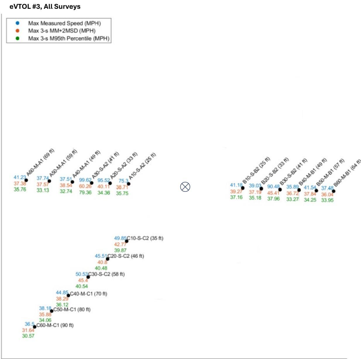
NOTE: The statistics shown are independent of each other. The maximums for any one sensor or specific statistic may not come from the same time window or the same survey.
Figure 26. eVTOL #3 Maximum Velocity Recorded at Each Sensor Across All Surveys in Plan View

Table 15. eVTOL #3 Maximum Velocity (mph) Recorded at Each Sensor Across All Surveys

Sensor ID	Distancefrom TLOFCenter (ft)	Max	Max 3-sMM	Max 3-sMM+2MSD	Max 3-sM95%
A10-S-A2	25	75.30	27.93	38.71	35.75
A20-S-A2	33	95.52	28.81	40.11	34.36
A30-S-A2	41	99.62	29.47	60.26	79.36
A40-M-A1	49	37.51	24.82	38.54	32.74
A50-M-A1	59	37.74	25.39	37.57	33.13
A60-M-A1	69	41.23	30.03	37.38	35.76
B10-S-B2	25	41.18	26.27	39.27	37.16
B20-S-B2	33	39.03	25.62	37.19	35.18
B30-S-B2	41	90.48	28.12	45.41	37.96
B40-M-B1	49	35.89	24.63	36.72	33.27
B50-M-B1	57	41.54	27.01	37.84	34.25
B60-M-B1	64	37.48	26.61	36.04	33.95
C10-S-C2	35	49.85	30.30	42.77	39.87
C20-S-C2	46	45.51	28.80	40.80	40.48
C30-S-C2	58	50.53	30.73	45.40	40.54
C40-M-C1	70	44.85	27.82	38.29	36.12
C50-M-C1	80	38.18	25.77	35.88	34.06
C60-M-C1	90	36.50	22.47	31.64	30.57

NOTE: The statistics shown are independent of each other. The maximums for any one sensor or specific statistic may not come from the same time window or the same survey.

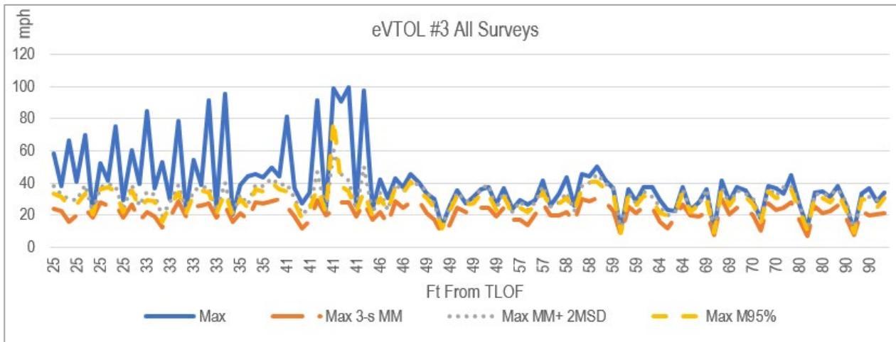
Figure 27. eVTOL #3 Line Graph of Maximum Velocity (mph) Recorded at Each Sensor for Each Survey (Sorted by Distance from TLOF Center from Left to Right)

6.3.2 eVTOL #3 Comparison to VVPM Modeling and Simulation

The VVPM simulations completed for the previous eVTOL aircraft revealed that the blade configuration of eVTOL #3 would likely pose a significant challenge to the hardware used for the VVPM simulation. An isolated multi-propeller model was created to conduct a systematic VVPM resolution study. Because particles are emitted from the trailing edge of the propeller blades, the blade spanwise locations for the particle emission (i.e., spanwise locations) can be adjusted to balance fidelity (i.e., fineness of spanwise discretization) and computational effort (i.e., more particles require more GPU memory and longer computation time). The fineness of discretization or distance between particle emission locations along the blade span is expressed in percent of propeller radius. Four particle resolutions were tested: 3% discretization over propeller blade (highest resolution), high-inboard/lower-outboard discretization, low-inboard/high-outboard discretization, and a constant 5% discretization (low resolution). The associated particle counts for the different discretizations and for isolated and full-aircraft mode are shown in Figure 28a. Obviously, the highest resolution had the largest number of particles for the same simulation duration of approximately 3.8 million. Simulation converged similarly for all particle resolutions and ,after approximately 10 revolutions, there was a noticeable difference in the predicted maximum velocity magnitude for the isolated propeller at a two-propeller diameter distance above the ground and the velocity measurement at a 1.35 propeller diameter distance from the center axis, see Figure 28b. Figure 28c shows the predicted velocity magnitude (x-axis) and the height above ground (y-axis). The different color lines represent the results for different VVPM resolutions. Similar to a CFD mesh sensitivity study, the results of this study were used for the DWOW simulation of the eVTOL #3 configuration.

Source Resolution*	Number of Particles
3% Full	3,713,580
0-0.7R (3%),0.7R-1R (5%)	2,628,072
0-0.85R (5%),0.85R-1R (3%)	2,171,016
5% Full	1,656,828

(a) Number of Particles for Different Resolutions

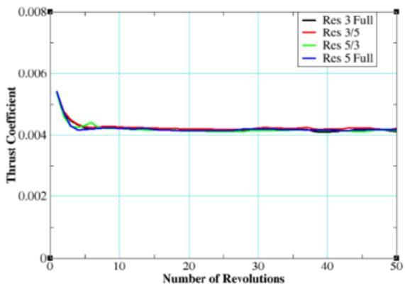
(b) Simulation Convergence for Different Resolutions

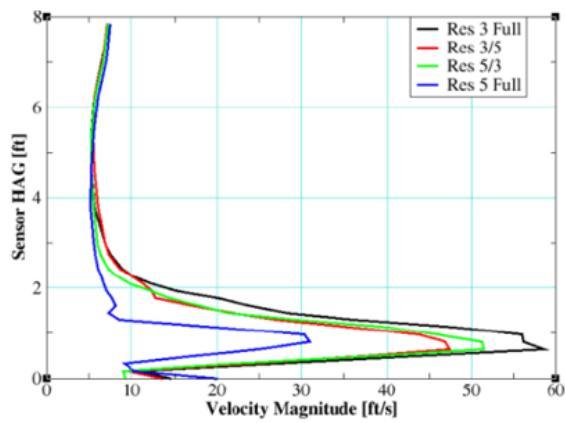
(c) Total Velocity Prediction for Different Resolutions
Figure 28. eVTOL #3 VVPM Resolution Sensitivity Study

The overall wake of eVTOL #3 is somewhat symmetric and characterized by significant aerodynamic interactions of the wakes of adjacent lift propellers. Exploratory velocity predictions were plotted at multiple locations along the 360°, 90°, 180°, and 270° radials. However, as detailed in the previous section, the sensors were not in these exact locations due to changes in the sensor array that came after the VVPM had been completed.

While the modeling included sensors closer to the aircraft and at four radials all separated by 90°, the actual survey included a completely different sensor configuration. This new configuration included three radials of sensors with more total sensor on each radial. This allowed for measurements farther away from the aircraft and beyond the aircraft’s associated SA, which were considered more important for determining vertiport design requirements. No attempt was made at simulation validation with this aircraft for several reasons:

1. The large number of propellers posed challenges with the limited graphics card capability at the time resulting in a lack of wake outside of the TLOF.

2. Data points measured with the new sensor configuration did not accurately follow the data points simulated.

3. The vertical sensor array was not included in the survey.

4. There were uncertainties in the geometry of the tested aircraft with respect to the simulation model due to lack of information on the aircraft available from the OEM.

6.4 eVTOL #4

DWOW of eVTOL #4 was not surveyed because it was not made available by the OEM, so there are no measurement findings to report. However, VVPM modeling was developed for it to determine if the limitations presented by the GPUs could be overcome with a hybrid approach. In this model, the overall flow field was divided into two domains: near field and far field. The near field was solved by VVPM, and the far field was evaluated based on flow mass flux conservation with regard to near field VVPM prediction (see Figure 29). The flow field sampling points are included in Figure 30.

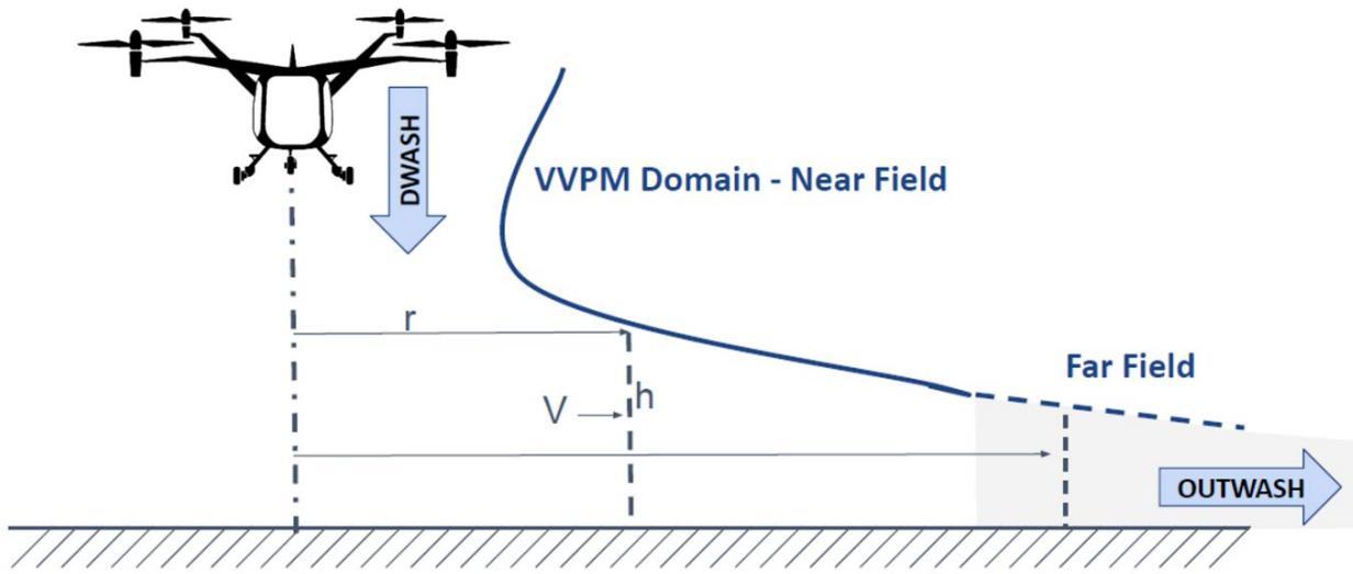
Figure 29. Hybrid Method

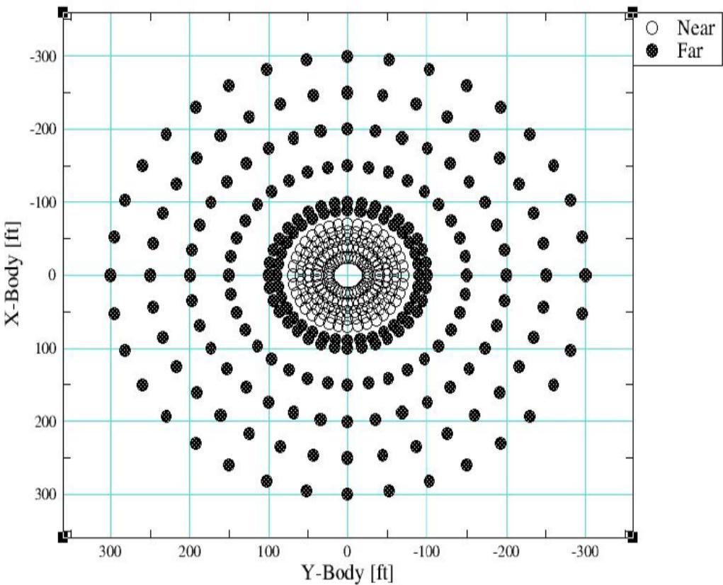
Figure 30. Flow Field Sampling Points

In-ground effect simulations were run with the rotor/propeller height of 20 ft above ground.
Figure 31 shows an example of the results of the model at a 90° radial from the aircraft.

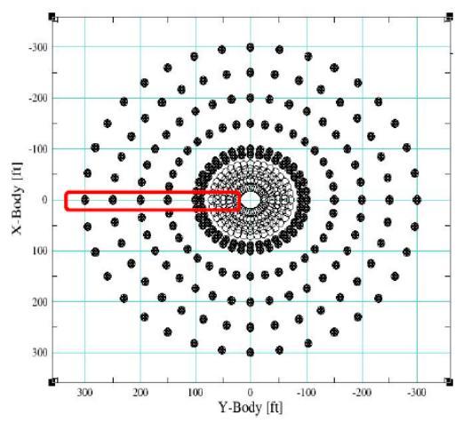
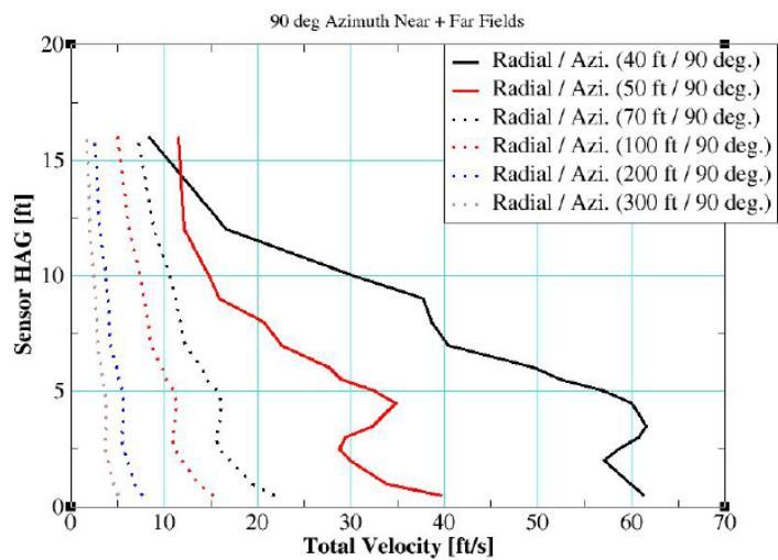
Figure 31. Velocity Profile at $9 0 ^ { \circ }$ Radial

Hybrid approach combines high-fidelity flow field predictions with analytical method to extend outwash velocity predictions into the far field. The next step would be to take surveys of an eVTOL #4 aircraft to compare with measured data.

7. CONCLUSIONS

The conclusions that follow are presented in two sections. The first section includes specific conclusions related to the modeling and simulation of the eVTOL aircraft with VVPM. The second section includes conclusions related to the velocity of DWOW measured and recorded during the surveys and general deductions associated with these velocities.

7.1 MODELING AND SIMULATION

eVTOL aircraft differ greatly in configuration and number of propellers. The large number of propellers makes it difficult to model much beyond what would be the safety area in EB 105. Based on the results presented and examined in this study, the following conclusions are drawn:

Aircraft geometry and property information is essential for building a simulation model capable of accurately predicting the DWOW profile. Important properties for the simulation model and for measuring correlation with measured data include propeller blade geometric planform (e.g., twist, chord distribution, root cutout), propeller radius, propeller hub locations, geometry, and location of blocking surfaces and bodies (e.g., wing, fuselage, tail surfaces). Most of this information was unavailable for much of this research.

The quality of correlation and associated demand on modeling properties for the simulation model varies for different eVTOL configurations with more accurate modeling data required for configurations with lift propellers in proximity to each other surface and parts of the aircraft.

Using a representative simulation based on manufacturer data allows the replay of the aircraft flight control histories modulating thrust for maintaining hover position rather than running constant speed simulation as an approximation.

Survey flight condition information (e.g., ambient wind, aircraft position/attitude, propeller speed, and thrust) is another important aspect for setting up VVPM simulation to closely reflect the real flight for accurate DWOW predictions.

For the eVTOL #2, the VVPM simulation results exhibited limited correlation with the measured data and captured some of the mean and minimum/maximum and the unsteadiness of the DWOW profile.

The proximity of the propellers can play an important role in the prediction of the DWOW profile. More specifically, the propellers operating near one another can induce strong aerodynamic interactions, which inherently affect the DWOW profile.

The vertical array is needed to get a fundamental understanding of the DWOW profile. As shown in horizontal array VVPM predictions, there were large changes in the velocity predictions even within 0.2-ft vertical variations in the sensor height. This is especially important given the unsteadiness of the flow captured both in the flight test and VVPM simulation.

• Some outfield sensors were not reached by the VVPM wake as the vortex particles retired from the simulation due to hardware memory constraints. While approximately 6 million particles were released into the simulation domain, which is presently the largest number of particles in any of the modeling team’s VVPM simulations, the newest memory cards were still not enough to model these particles at SA and beyond. These current limitations make VVPM alone an unlikely method for forecasting where people and property will not be affected by high winds. However, a more recent development augmenting VVPM with global mass conservation could provide valuable insight into predicting the outwash beyond the safety area at any outfield location of interest. This methodology leverages the VVPM solution in the near field regions to predict the farther outfield sensor outwash using the principle of global mass conservation.

7.2 DWOW VELOCITIES

The FAA’s Rotorwash Analysis Handbook indicates that most rotorwash-related mishaps can be avoided if separation distances are maintained so that impacting rotorwash-generated velocities do not exceed 30 to 40 knots (34.5–46 mph) across the ground (Ferguson, 1994).

The highest DWOW velocities measured for each eVTOL aircraft surveyed—all under 6,500 lb—by distance from the TLOF center, reveal that the DWOW at the SA for that aircraft based on EB 105 and beyond often surpass 34.5 mph (see Table 16).

Table 16. Highest DWOW Velocity (mph) Measured

Aircraft	DistancefromTLOFCenter (ft)	Max	Max 3-sMM	Max 3-sMM+2MSD	MaxM95%
eVTOL #1	23	99.32	50.09	88.06	83.59
	28	98.72	45.39	79.91	70.29
	33	82.88	42.86	66.59	65.38
	46	83.18	38.09	68.69	65.86
	69	55.1	26.46	42.03	40.08
eVTOL #2	37	98.49	49.58	71.10	68.73
	38	91.15	39.11	69.06	64.03
	50	93.63	47.26	75.22	62.83
	53	84.72	44.87	77.62	66.00
	58	99.24	46.81	85.13	69.71
	71	67.85	41.20	71.45	59.63
	75	68.81	42.41	69.54	58.46
	82	85.90	40.92	69.96	58.97
	85	65.96	40.73	68.41	59.36
	95	73.52	41.33	70.24	63.73
	106	62.35	37.65	65.71	59.27
	116	65.04	36.43	63.57	57.04
	126	69.03	38.78	65.09	63.96
eVTOL #3	25	75.30	27.93	39.27	37.16
	33	95.52	28.81	40.11	35.18
	35	49.85	30.3	42.77	39.87
	41	99.62	29.47	60.26	79.36
	46	45.51	28.8	40.8	40.48

Aircraft	DistancefromTLOFCenter (ft)	Max	Max 3-sMM	Max 3-sMM+2MSD	MaxM95%
	49	37.51	24.82	38.54	33.27
	57	41.54	27.01	37.84	34.25
	58	50.53	30.73	45.4	40.54
	59	37.74	25.39	37.57	33.13
	64	37.48	26.61	36.04	33.95
	69	41.23	30.03	37.38	35.76
	70	44.85	27.82	38.29	36.12
	80	38.18	25.77	35.88	34.06
	90	36.5	22.47	31.64	30.57

Note: The statistics shown are independent of each other. The maximums for any one sensor or specific statistic may not come from the same time window or the same survey.

As shown in Figure 32, while the highest DWOW velocity measured was generally closer to the TLOF center, it does not slow below dangerous thresholds at the sensors farther away. As the eVTOL approaches and departs the TLOF, its DWOW will travel with the aircraft. Additionally, the velocity of the air is strong and turbulent, creating a chaotic area that takes time to dissipate. These findings are dependent on the position and maneuvering of the aircraft.

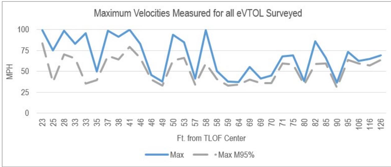
Figure 32. Maximum Velocity (mph) Measured by Sensor Distance to TLOF Center for All eVTOL Aircraft Surveyed
The overall maximum speeds and maximum speeds by distance categories are shown in Table 17.

Table 17. Overall Maximum Speeds Measured for All eVTOL Aircraft

Overall Maximum	Speed (mph)
Instant Max (mph)	99.62 at 41 ft from TLOFCenter
Max 3-s M95% (mph)	83.59 at 23 ft from TLOFCenter
Maximum by Distance to TLOFCenter (ft)	Instant Max (mph)
0-25	99.32
26-50	99.62
51-75	99.24
76-100	85.90
101-125	65.04
125+	69.03
Maximum by Distance to TLOFCenter (ft)	Max 3-s M95% (mph)
0-25	83.59
26-50	79.36
51-75	66.00
76-100	63.73
101-25	59.27
125+	63.96

The maximum velocities observed during these surveys varied from survey to survey and from aircraft to aircraft. The novel designs and complex wake-to-wake interaction, wake-tofuselage interaction, and wake-to-ground interaction—all changing depending on aircraft speed, heading, and altitude—result in non-uniform and high-velocity DWOW flow fields that can easily go beyond the safety area of a vertiport. In confined areas, these flow fields could also be impacted by structures on the ground that were not present in this research design. Additional research is required on unique aircraft designs and environments.

Conclusions drawn from the DWOW velocities on prototype eVTOL are summarized as follows:

eVTOL aircraft DWOW at the SA and beyond surpass most of the air velocity sensitivity thresholds found in AC 150/5300-13B, Airport Design (FAA, 2024), and in the FAA Rotorwash Analysis Handbook (Ferguson, 1994) (34.5 mph).

The highest instantaneous maximum velocity measured was approximately 100 mph at 41 ft from the TLOF center. The highest M95% was 84 mph at 23 ft from the TLOF center. The highest speed measured beyond the SA for all the aircraft was more than 85 mph at 82 ft from the TLOF center. Speeds of more than 60 mph were measured at 100 ft from the TLOF center.

While the maximum M95% are lower than the instantaneous maximums measured, instantaneous winds can be more upsetting for people than sustained winds due to a phenomenon known as the “startle response.”

Regardless of how the speeds are analyzed (instantaneous maximum vs 3-sec M95%), eVTOL aircraft have high-velocity DWOW that will impact people and property on the ground. This not only includes people and property on the vertiport but possibly people and property outside of the vertiport boundaries.

The high-velocity DWOW of eVTOL aircraft should be considered when designing a vertiport because it has the potential to create safety risks to people, aircraft, equipment, and infrastructure, on and off the vertiport.

Under 14 C.F.R. Part 157, the FAA will be required to make an airspace determination on most new vertiports (Notice of Construction, Alteration, Activation, and Deactivation of Airports, 1991). This determination considers the safety of persons and property on the ground, and DWOW can have a detrimental effect on them. Accordingly, DWOW should be mitigated through either vertiport design features or operational procedures. This can be accomplished by the establishment of a DCA. The area can be operational in nature where DWOW velocity exceeds 34.5 mph, and it should move with the aircraft as it maneuvers.

8. REFERENCES

Australian Transport Safety Bureau. (2023). Downwash incidents at hospital helicopter landing sites (Investigation Number AD-2022-001). https://www.atsb.gov.au/publications/research-and-analysis-report/2023/downwashincidents-hospital-helicopter-landing-sites

Brown, R. E. (2023, September 5–7). Do eVTOL aircraft create an inherently more problematic downwash than conventional helicopters? [Paper presentation]. 49th European Rotorcraft Forum 2023, Buckeburg, Germany. https://sophrodyneaerospace.com/static/soph_aerospace/files/downloads/Sophrodyne_eVTOL_Downwa sh.pdf

Cleveland Clinic. (2023). Amygdala. https://my.clevelandclinic.org/health/body/24894- amygdala

Federal Aviation Administration (FAA). (2017). Upset prevention and recovery training (Advisory Circular [AC] 120-111). U.S. Department of Transportation, Federal Aviation Administration. https://www.faa.gov/regulations_policies/advisory_circulars/index.cfm/go/document.i nformation/documentID/1027328

FAA. (2023a, March 13). Vertiport design (FAA Engineering Brief [EB] 105). U.S. Department of Transportation, Federal Aviation Administration. https://www.faa.gov/airports/engineering/engineering_briefs/engineering_brief_105_ vertiport_design

FAA. (2023b, April 26). Urban air mobility concept of operations, v2.0. Federal Aviation Administration. https://www.faa.gov/sites/faa.gov/files/Urban%20Air%20Mobility%20%28UAM%29 %20Concept%20of%20Operations%202.0_0.pdf

FAA. (2024). Airport design (AC 150/5300-13B). U.S. Department of Transportation, Federal Aviation Administration. https://www.faa.gov/regulations_policies/advisory_circulars/index.cfm/go/document.i nformation/documentID/1040834

Ferguson, S. (1994). Rotowash analysis handbook, Volume I - Development and Analysis (DOT/FAA/RD-93/31,I). U.S. Department of Transportation, Federal Aviation Administration. https://archive.org/details/DTIC_ADA283719/mode/2up

Goodrich, K., & Theodore, C. (2021, January 11–21). Description of the NASA Urban Air Mobility Maturity Level (UML) scale [Paper presentation]. American Institute of Aeronautics and Astronautics (AIAA) SciTech Forum, Virtual. https://ntrs.nasa.gov/api/citations/20205010189/downloads/UML%20Paper%20SciTe ch%202021.pdf

KABC Television. (2022). 3 children hurt at Rancho Cucamonga Police event involving a sheriff's helicopter, bounce house. ABC7.com. https://abc7.com/rancho-cucamongachildren-hurt-bounce-house-sheriffs-helicopter/11812717/

Lee, H., Sengupta, B., Araghizadeh, M., & Myong, R. (2022). Review of vortex methods for rotor aerodynamics and wake dynamics. Advances in Aerodynamics, 4(20). https://doi.org/10.1186/s42774-022-00111-3

National Aeronautics and Space Administration (NASA). (2020, November). Advanced air mobility (AAM) vertiport automation trade study. https://ntrs.nasa.gov/api/citations/20210009757/downloads/20210009757_MAJohnso n_VertiportTradeStudy_final.pdf

National Oceanic and Atmospheric Administration (NOAA), National Weather Service Storm Prediction Center. (2023). Beaufort wind scale. https://www.spc.noaa.gov/faq/tornado/beaufort.html

Notice of Construction, Alteration, Activation, and Deactivation of Airports.14 C.F.R. § 157. (1991). https://www.ecfr.gov/current/title-14/chapter-I/subchapter-I/part-157

Preston, J., Troutman, S., Keen, E., Silva, M., Whitman, N., & Ferguson, S. (2014). Rotorwash operational footprint modeling (Technical Report RDMR-AF-14-02). U.S. Army Research, Development and Engineering Command (RDECOM). https://ntrl.ntis.gov/NTRL/dashboard/searchResults/titleDetail/ADA607614.xhtml

Starkenburg, D., Metzger, S., Fochesatto, G., Alfieri, J., Gens, R., Prakash, A., & Cristóbal, J. (2016). Assessment of despiking methods for turbulence data in micrometeorology. Journal of Atmospheric and Oceanic Technology, 33(9), 2001–2013. https://doi.org/10.1175/JTECH-D-15-0154.1

Swarts, P. (2016). Air National Guard helicopter downwash led to hiker injury in 2014 rescue. Air Force Times. https://www.airforcetimes.com/2016/08/16/air-nationalguard-helicopter-downwash-led-to-hiker-injury-in-2014-rescue-report/

Werfelman, L. (2023). Fatal downwash. Flight Safety Foundation. https://flightsafety.org/asw-article/fatal-downwash/